Calculating the Optimal Step in Shift-Reduce Dependency Parsing:
From Cubic to Linear Time
Mark-Jan Nederhof
School of Computer Science University of St Andrews, UK
Abstract
We present a new cubic-time algorithm to calculate the optimal next step in shift-reduce dependency parsing, relative to ground truth, commonly referred to as dynamic oracle. Un-like existing algorithms, it is applicable if the training corpus contains non-projective struc-tures. We then show that for a projective training corpus, the time complexity can be improved from cubic to linear.
1 Introduction
A deterministic parser may rely on a classifier that predicts the next step, given features extracted from the present configuration (Yamada and Matsumoto, 2003; Nivre et al., 2004). It was found that accuracy improves if the classifier is trained not just on configurations that correspond to the ground-truth, or ‘‘gold’’, tree, but also on configurations that a parser would typically reach when a classifier strays from the optimal predictions. This is known as adynamic oracle.1
The effective calculation of the optimal step for some kinds of parsing relies on ‘arc-decomposibility’, as in the case of Goldberg and Nivre (2012, 2013). This generally requires a projective training cor-pus; an attempt to extend this to non-projective training corpora had to resort to an approxima-tion (Aufrant et al., 2018). It is known how to calculate the optimal step for a number of
non-1A term we avoid here, as dynamic oracles are neither oracles nor dynamic, especially in our formulation, which allows gold trees to be non-projective. Following, for example, Kay (2000), an oracle informs a parser whether a step may lead to the correct parse. If the gold tree is non-projective and the parsing strategy only allows projective trees, then there are no steps that lead to the correct parse. At best, there is an optimal step, by some definition of optimality. An algorithm to compute the optimal step, for a given configuration, would typically not change over time, and therefore is not dynamic in any generally accepted sense of the word.
projective parsing algorithms, however (G´omez-Rodr´ıguez et al., 2014; G´omez-(G´omez-Rodr´ıguez and Fern´andez-Gonz´alez, 2015; Fern´andez-Gonz´alez G´omez-Rodr´ıguez, 2018a); see also de Lhoneux et al. (2017).
Ordinary shift-reduce dependency parsing is known at least since Fraser (1989); see also Nasr (1995). Nivre (2008) calls it ‘‘arc-standard parsing.’’ For shift-reduce dependency parsing, calculation of the optimal step is regarded to be difficult. The best known algorithm is cubic and is only applicable if the training corpus is projective (Goldberg et al., 2014). We present a new cubic-time algorithm that is also applicable to non-projective training corpora. Moreover, its architecture is modular, expressible as a generic tabular algorithm for dependency parsing plus a context-free grammar that expresses the allow-able transitions of the parsing strategy. This dif-fers from approaches that require specialized tabular algorithms for different kinds of parsing (G´omez-Rodr´ıguez et al., 2008; Huang and Sagae, 2010; Kuhlmann et al., 2011).
The generic tabular algorithm is interesting in its own right, and can be used to determine the opti-mal projectivization of a non-projective tree. This is not to be confused with pseudo-projectivization (Kahane et al., 1998; Nivre and Nilsson, 2005), which generally has a different architecture and is used for a different purpose, namely, to allow a projective parser to produce non-projective structures, by encoding non-projectivity into pro-jective structures before training, and then recon-structing potential non-projectivity after parsing.
A presentational difference with earlier work is that we do not define optimality in terms of ‘‘loss’’ or ‘‘cost’’ functions but directly in terms of attain-able accuracy. This perspective is shared by Straka et al. (2015), who also relate accuracies of compet-ing steps, albeit by means of actual parser output and not in terms of best attainable accuracies.
283
We further show that if the training corpus is projective, then the time complexity can be reduced to linear. To achieve this, we develop a new approach of excluding computations whose accuracies are guaranteed not to exceed the accu-racies of the remaining computations. The main theoretical conclusion is that arc-decomposibility is not a necessary requirement for efficient cal-culation of the optimal step.
Despite advances in unrestricted non-projective parsing, as, for example, Fern´andez-Gonz´alez and G´omez-Rodr´ıguez (2018b), many state-of-the-art dependency parsers are projective, as, for example, Qi and Manning (2017). One main practical contribution of the current paper is that it introduces new ways to train projective parsers using non-projective trees, thereby enlarging the portion of trees from a corpus that is available for training. This can be done either after applying optimal projectivization, or by computing optimal steps directly for non-projective trees. This can be expected to lead to more accurate parsers, especially if a training corpus is small and a large proportion of it is non-projective.
2 Preliminaries
In this paper, aconfiguration(for sentence length n) is a 3-tuple (α, β, T) consisting of a stack α, which is a string of integers each between 0 andn, aremaining inputβ, which is a suffix of the string
1 · · · n, and a set T of pairs (a, a0) of integers, with 0 ≤a≤ nand1 ≤a0 ≤n. Further,αβ is a subsequence of 0 1 · · · n, starting with 0. Integer 0 represents an artificial input position, not corresponding to any actual token of an input sentence.
An integer a0 (1 ≤ a0 ≤ n) occurs as second element of a pair (a, a0) ∈ T if and only if it does not occur in αβ. Furthermore, for each a0 there is at most one a such that (a, a0) ∈ T. If
(a, a0)∈Tthena0is generally called adependent
ofa, but as we will frequently need concepts from graph theory in the remainder of this article, we will consistently call a0 a child of a and a the
parentofa0; ifa0 < athena0is aleft childand if a < a0then it is aright child. The terminology is extended in the usual way to includedescendants
and ancestors. Pairs (a, a0) will henceforth be callededges.
For sentence lengthn, theinitial configuration
is (0,1 2 · · · n,∅), and a final configuration is
shift:
(α, bβ, T)`(αb, β, T)
reduce left:
(αa1a2, β, T)`(αa1, β, T ∪ {(a1, a2)}) reduce right:
(αa1a2, β, T)`(αa2, β, T ∪ {(a2, a1)}), provided|α|>0
Table 1: Shift-reduce dependency parsing.
of the form(0, ε, T), whereεdenotes the empty string. The three transitions of shift-reduce de-pendency parsing are given in Table 1. By step
we mean the application of a transition on a particular configuration. Bycomputationwe mean a series of steps, the formal notation of which uses `∗, the reflexive, transition closure of`. If (0,1 2 · · · n,∅)`∗(0, ε, T), thenT represents a
tree, with 0 as root element, andT isprojective, which means that for each node, the set of its descendants (including that node itself) is of the form{a, a+ 1, . . . , a0−1, a0}, for someaanda0. In general, adependency treeis any tree of nodes labelled 0, 1, . . . ,n, with 0 being the root.
The score of a tree T for a sentence is the number of edges that it has in common with a given gold treeTg for that sentence, or formally
|T ∩Tg|. Theaccuracyis the score divided byn.
Note that neither tree need be projective for the score to be defined, but in this paper the first tree, T, will normally be projective. Where indicated, alsoTg is assumed to be projective.
Assume an arbitrary configuration (α, β, T)
for sentence length n and assume a gold tree Tg for a sentence of that same length, and
as-sume three steps (α, β, T) ` (αi, βi, Ti), with
i = 1,2,3, obtainable by a shift, reduce left
or reduce right, respectively. (If β = ε, or |α| ≤ 2, then naturally some of the three transitions need to be left out of consideration.) We now wish to calculate, for each ofi= 1,2,3, the maximum value of|Ti0∩Tg|, for anyTi0 such
that (αi, βi, Ti) `∗ (0, ε, Ti0). For i = 1,2,3, let
σibe this maximum value. The absolute scoresσi
are strictly speaking irrelevant; the relative values determine which is the optimal step, or whichare
the optimal steps, to reach a tree with the highest score. Note that|{i|σi = maxjσj}|is either 1,
2, or 3. In the remainder of this article, we find it more convenient to calculateσi− |T ∩Tg|for
We can put restrictions on the set of allowable computations (α, β, T) `∗ (0, ε, T ∪ T0). The left-before-right strategy demands that all edges
(a, a0) ∈ T0 with a0 < a are found before any edges(a, a0) ∈T0 witha < a0, for eachathat is rightmost inαor that occurs inβ. Thestrict left-before-right strategy in addition disallows edges
(a, a0) ∈ T0 with a0 < a for each a in α other than the rightmost element. The intuition is that a non-strict strategy allows us to correct mistakes already made: If we have already pushed other elements on top of a stack elementa, thenawill necessarily obtain right children before it occurs on top of the stack again, when it can take (more) left children. By contrast, the strict strategy would not allow these left children.
The definition of theright-before-leftstrategy is symmetric to that of the left-before-right strategy, but there is no independent strict right-before-left strategy. In this paper we consider all three strategies in order to emphasize the power of our framework. It is our understanding that Goldberg et al. (2014) does not commit to any particular strategy.
3 Tabular Dependency Parsing
We here consider context-free grammars (CFGs) of a special form, with nonterminals inN∪(N`×
Nr), for appropriate finite setsN,N`,Nr, which
need not be disjoint. The finite set of terminals is denotedΣ. There is a single start symbolS ∈N. Rules are of one of the forms:
• (B, C)→a,
• A→(B, C),
• (B0, C)→A(B, C),
• (B, C0)→(B, C)A,
where A∈ N,B, B0 ∈N`, C, C0 ∈ Nr,a ∈Σ.
A first additional requirement is that if(B0, C)→ A (B, C) is a rule, then(B0, C0) → A (B, C0), for anyC0 ∈Nr, is also a rule, and if(B, C0) →
(B, C) A is a rule, then(B0, C0) → (B0, C) A, for any B0 ∈ N`, is also a rule. This justifies
our notation of such rules in the remainder of this paper as (B0, ) → A (B, ) and ( , C0) →
( , C) A, respectively. These two kinds of rules correspond to attachment of left and right children, respectively, in dependency parsing. Secondly, we require that there is precisely one rule(B, C)→a for eacha∈Σ.
W`(B, i, i) =
1, if(B, C)→ai
0, otherwise
Wr(C, i, i) =
1, if(B, C)→ai
0, otherwise
W`(B, C, i, j) =LkWr(B, i, k)⊗
W`(C, k+ 1, j)⊗w(j, i) Wr(B, C, i, j) =LkWr(B, i, k)⊗
W`(C, k+ 1, j)⊗w(i, j) W`(C0, i, j) =LA→(D,B),(C0,)→A(C,), k
W`(D, i, k)⊗W`(B, C, k, j) Wr(B0, i, j) =L(,B0)→(,B)A, A→(C,D), k
Wr(B, C, i, k)⊗Wr(D, k, j)
W =L
S→(B,C)W`(B,0,0)⊗Wr(C,0, n)
Table 2: Weighted parsing, for an arbitrary semi-ring, with0≤i < j ≤n.
Note that the additional requirements make the grammar explicitly ‘‘split’’ in the sense of Eisner and Satta (1999), Eisner (2000), and Johnson (2007). That is, the two processes of attaching left and right children, respectively, are independent, with rules (B, C) → a creating ‘‘initial states’’ B and C, respectively, for these two processes. Rules of the form A → (B, C) then combine the end results of these two processes, possibly placing constraints on allowable combinations of BandC.
To bring out the relation between our subclass of CFGs and bilexical grammars, one could ex-plicitly write(B, C)(a)→a,A(a)→(B, C)(a),
(B0, )(b) → A(a) (B, )(b), and ( , C0)(c) →
( , C)(c)A(a).
Purely symbolic parsing is extended to weighted parsing much as usual, except that instead of attaching weights to rules, we attach a scorew(i, j)
to each pair(i, j), which is a potential edge. This can be done for any semiring. In the semiring we will first use, a value is either a non-negative integer or−∞. Further,w1⊕w2 = max(w1, w2) andw1⊗w2 =w1+w2ifw1 6=−∞andw26= −∞andw1⊗w2=−∞otherwise. Naturally, the identity element of⊕is0=−∞and the identity element of⊗is1= 0.
Tabular weighted parsing can be realized following Eisner and Satta (1999). We assume the input is a string a0a1· · ·an ∈ Σ∗, with a0 being the prospective root of a tree. Table 2 presents the cubic-time algorithm in the form of a system of recursive equations. With the semiring we chose above, W`(B, i, j)represents
(S, S) → a
S → (S, S)
( , S) → (, S)S
[image:4.595.370.467.58.184.2](S, ) → S(S, )
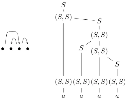
[image:4.595.136.223.60.104.2]Table 3: Grammar for projective dependency parsing, withΣ ={a}andN =N`=Nr={S}.
Figure 1: Dependency structure and corresponding parse tree that encodes a computation of a shift-reduce parser.
A1· · ·Am(Bm, ) ⇒ A1· · ·Amaj ⇒∗ ai· · ·aj,
for some m ≥0, andWr(C, i, j)has symmetric
meaning. Intuitively,W`(B, i, j)considersajand
its left dependents and Wr(C, i, j) considers ai
and its right dependents. A value W`(B, C, i, j),
or Wr(B, C, i, j), represents the highest score
combiningaiand its right dependents andaj and
its left dependents, meeting in the middle at some k, including also an edge from ai toaj, or from
ajtoai, respectively.
One may interpret the grammar in Table 3 as encoding all possible computations of a shift-reduce parser, and thereby all projective trees. As there is only one way to instantiate the under-scores, we obtain rule(S, S) →(S, S) S, which corresponds to reduce left, and rule (S, S) → S(S, S), which corresponds toreduce right.
Figure 1 presents a parse tree for the grammar and the corresponding dependency tree. Note that if we are not given a particular strategy, such as left-before-right, then the parse tree underspec-ifies whether left children or right children are attached first. This is necessarily the case because the grammar is split. Therefore, the computation in this example may consist of threeshifts, fol-lowed by onereduce left, one reduce right, and one reduce left, or it may consist of two
shifts, one reduce right, one shift, and two
reduce lefts.
(P, P) → p
(S, S) → s
P → (P, P)
S → (P, S)
S → (S, S)
(S, ) → P(S, )
(S, ) → S(S, )
(, S) → (, P)S
(, S) → (, S)S
(S, ) → P(P, )
Table 4: Grammar for dependency parsing of pksm+1, representing a stack of lengthk+ 1and remaining input of length m, with Σ = {p, s}, N =Nr =N` ={P, S}. The last rule would be
excluded for the strict left-to-right strategy, or alternatively one can set w(i, j) = −∞ for j < i < k.
For a given gold treeTg, which may or may not
be projective, we letw(i, j) =δg(i, j), where we
defineδg(i, j) = 1if(i, j)∈Tg andδg(i, j) = 0
otherwise. With the grammar from Table 3, the value W found by weighted parsing is now the score of the most accurate projective tree. By backtracing from W as usual, we can construct the (or more correctly, a) tree with that highest accuracy. We have thereby found an effective way to projectivize a treebank in an optimal way. By a different semiring, we can count the number of trees with the highest accuracy, which reflects the degree of ‘‘choice’’ when projectivizing a treebank.
4 OOO(n(n(n333)))Time Algorithm
In a computation starting from a configuration
(a0· · ·ak, b1· · ·bm, T), not every projective parse
of the stringa0· · ·akb1· · ·bm is achievable. The
structures that are achievable are captured by the grammar in Table 4, withP for prefix andS for suffix (also for ‘‘start symbol’’). NonterminalsP and(P, P)correspond to a node ai (0 ≤ i < k)
that does not have children. Nonterminal S corresponds to a node that has eitherak or some
bj (1≤j≤m) among its descendants. This then
means that the node will appear on top of the stack at some point in the computation. Nonterminal
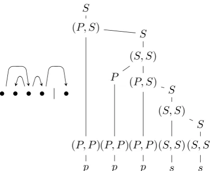
[image:4.595.71.288.145.318.2]Figure 2: Dependency structure and corresponding parse tree, for stack of height 4 and remaining input of length 1.
Nonterminal (P, S) corresponds to a node ai
(0 ≤ i < k) that has ak among its descendants
but that does not have a left child. Nonterminal
(S, P)corresponds to a nodeai (0≤ i < k) that
has a left child but no right children. Foraito be
given a left child, it is required that it eventually appear on top of the stack. This requirement is encoded in the absence of a rule with right-hand side (S, P). In other words, (S, P) cannot be part of a successful derivation, unless the rule
(S, S) → (S, P) S is subsequently used, which then corresponds to givingaia right child that has
akamong its descendants.
Figure 2 shows an example. Note that we can partition a parse tree into ‘‘columns’’, each con-sisting of a path starting with a label inN, then a series of labels in N`×Nr and ending with a
label inΣ.
A dependency structure that is not achievable, and that appropriately does not correspond to a parse tree, for a stack of height 4 and remaining input of length 1, is:
• • • • | •
Suppose we have a configuration (a0· · ·ak,
b1· · ·bm, T)for sentence lengthn, which implies
k+m ≤n. We need to decide whether ashift,
reduce left, orreduce right should be done in order to achieve the highest accuracy, for given gold tree Tg. For this, we calculate three values
σ1,σ2andσ3, and determine which is highest.
The first value σ1 is obtained by investigat-ing the configuration (a0· · ·akb1, b2· · ·bm,∅)
resulting after a shift. We run our generic tab-ular algorithm for the grammar in Table 4, for input pk+1sm, to obtain σ1 = W. The scores are obtained by translating indices of a0· · · akb1· · ·bm = c0· · ·ck+m to indices in the
orig-inal input, that is, we let w(i, j) = δg(ci, cj).
However, the shift, which pushes an element on top ofak, implies thatakwill obtain right children
before it can obtain left children. If we assume the left-before-right strategy, then we should avoid that ak obtains left children. We could do that
by refining the grammar, but find it easier to set w(k, i) =−∞for alli < k.
For the second valueσ2, we investigate the con-figuration(a0· · ·ak−1, b1· · ·bm,∅)resulting after
areduce left. The same grammar and algorithm are used, now for input pk−1sm+1. With a0· · · ak−1b1· · ·bm = c0· · ·ck+m−1, we let w(i, j) =
δg(ci, cj). We let σ2 = W ⊗ δg(ak−1, ak). In
case of a strict left-before-right strategy, we set w(k−1, i) = −∞ for i < k−1, to avoid that ak−1 obtains left children after having obtained a right childak.
If k ≤ 1 then the third value is σ3 = −∞, as noreduce rightis applicable. Otherwise we investigate(a0· · ·ak−2ak, b1· · ·bm,∅). The same
grammar and algorithm are used as before, and w(i, j) =δg(ci, cj)witha0· · ·ak−2akb1· · ·bm=
c0· · ·ck+m−1. Now σ3 = W ⊗ δg(ak, ak−1). In case of a right-before-left strategy, we set w(k, i) =−∞fork < i.
We conclude that the time complexity of cal-culating the optimal step is three times the time complexity of the algorithm of Table 2, hence cubic inn.
Figure 3: A nodeνwith label inN`×Nrtranslates to
configuration( ¯d1· · ·d¯k0,¯e1· · ·e¯m0, T), via its shortest
path to the root. The overlined symbols denote the integers between 0 and n corresponding to d1· · ·
dk0e1· · ·em0 ∈p+s∗.
a bijection between parse trees and computations. For example, in the middle column of the parse tree in Figure 2, the(P, S)and its right child occur below the(S, S)and its left child, to indicate the
reduce leftprecedes thereduce right. The proof in one direction assumes a parse tree, which is traversed to gather the steps of a computation. This traversal is post-order, from left to right, but skipping the nodes representing stack elements below the top of the stack, starting from the leftmost node labeled s. Each node ν with a label in N`×Nr corresponds to a step.
If the child of ν is labeled s, then we have a
shift, and if it has a right or left child with a label in N, then it corresponds to a reduce left or
reduce right, respectively. The configuration resulting from that step can be constructed as sketched in Figure 3. We follow the shortest path from ν to the root. All the leaves to the right of the path correspond to the remaining input. For the stack, we gather the leaves in the columns of the nodes on the path, as well as those of the left children of nodes on the path. Compare this with the concept of right-sentential forms in the theory of context-free parsing.
For a proof in the other direction, we can make use of existing parsing theory, which tells us how to translate a computation of the shift-reduce parser to a dependency structure, which in turn is easily translated to an undecorated parse tree. It then remains to show that the nodes in that tree can be decorated (in fact in a unique way), according to the rules from Table 4. This is straightforward given the meanings ofP andS described earlier in this section. Most notably, the absence of a rule
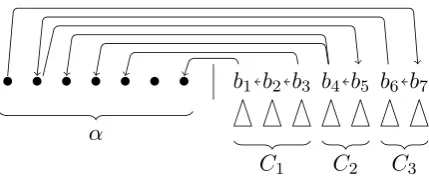
Figure 4: ComponentsC1,C2,C3partitioning nodes in
β, and gold edges linking them toα.
with right-hand side ( , P) P does not prevent the decoration of a tree that was constructed out of a computation, because a reduction involving two nodes within the stack is only possible if the rightmost of these nodes eventually appears on top of the stack, which is only possible when the computation has previously madeaka descendant
of that node, hence we would have S rather thanP.
5 OOO(n(n(n222)Time Algorithm
Assume a given configuration(α, β, T)as before, resulting from a shift or reduction. Let α =
a0· · ·ak, A = {a0, . . . , ak}, and let B be the
set of nodes in β. We again wish to calculate the maximum value of|T0∩Tg|for anyT0 such
that (α, β,∅) `∗ (0, ε, T0), but now under the
assumption thatTg is projective. Let us call this
value σmax. We define w in terms of δg as in
the previous section, setting w(i, j) = −∞ for an appropriate subset of pairs (i, j) to enforce a strategy that is (non-)strict left-before-right or right-before-left.
The edges in Tg ∩(B ×B) partition the
re-maining input into maximal connected compo-nents. Within these components, a node b ∈ B is called criticalif it satisfies one or both of the following two conditions:
• At least one descendant of b (according to Tg) is not inB.
• The parent ofb(according toTg) is not inB.
LetBcrit ⊆ B be the set of critical nodes, listed
in order asb1, . . . , bm, and letBncrit =B\Bcrit.
Figure 4 sketches three components as well as edges inTg∩(A×B)andTg∩(B×A).
Com-ponent C1, for example, contains the critical elements b1, b2, and b3. The triangles under b1, . . . , b7 represent subtrees consisting of edges leading to non-critical nodes. For eachb∈Bcrit,
[image:6.595.74.291.58.189.2]critical nodes have zero or more children in the stack. Further, if(a, b) ∈Tg∩(A×Bcrit), then
b is the rightmost critical node in a component; examples areb5andb7in the figure.
Let Tmax be any tree such that (α, β,∅) `∗
(0, ε, Tmax)and|Tmax∩Tg|=σmax. Then we can
find another treeTmax0 that has the same properties
and in addition satisfies:
1. Tg∩(B×Bncrit)⊆Tmax0 ,
2. Tmax0 ∩(Bncrit ×A) =∅,
3. Tmax0 ∩(B×Bcrit)⊆Tg,
or in words, (1) the subtrees rooted in the critical nodes are entirely included, (2) no child of a non-critical node is in the stack, and (3) within the remaining input, all edges to critical nodes are gold. Very similar observations were made before by Goldberg et al. (2014), and therefore we will not give full proofs here. The structure of the proof is in each case that all violations of a property can be systematically removed, by rearranging the computation, in a way that does not decrease the score.
We need two more properties:
4. If (a, b) ∈ Tmax0 ∩(A×Bcrit) \ Tg then
either:
• b is the rightmost critical node in its component, or
• there is (b, a0) ∈ Tmax0 ∩Tg, for some
a0 ∈ A and there is at least one other critical node b0 to the right ofb, but in the same component, such that(b0, a00)∈ Tmax0 ∩Tg or(a00, b0) ∈ Tmax0 ∩Tg, for
somea00 ∈A.
5. If(b, a)∈Tmax0 ∩(Bcrit×A) \ Tgthen there
is(b, a0)∈Tmax0 , for somea0 ∈A, such that
a0is a sibling ofaimmediately to its right.
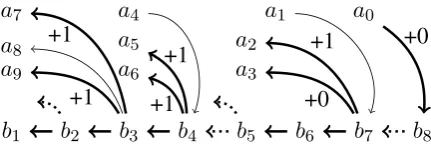
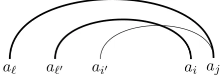
Figure 5, to be discussed in more detail later, illustrates property (4) for the non-gold edge from a4; this edge leads to b4 (which has outgoing gold edge toa5) rather than tob5orb6. It further respects property (4) because of the gold edges connected to b7 and b8, which occur to the right ofb4 but in the same component. Property (5) is illustrated for the non-gold edge from b3 to a8, which has siblinga9immediately to the right.
[image:7.595.308.524.55.129.2]The proof that property (4) may be assumed to hold, without loss of generality, again involves
Figure 5: Counting additional gold edges inA×Bcrit∪ Bcrit ×A. Gold edges are thick, others are thin. Gold
edges that are not created appear dotted.
making local changes to the computation, in particular replacing the b in an offending non-gold edge (a, b) ∈ A×Bcrit by another critical
node b0 further to the left or at the right end of the component. Similarly, for property (5), if we have an offending non-gold edge (b, a), then we can rearrange the computation, such that nodeais reduced not intobbut into one of the descendants ofbinB that was given children inA. If none of the descendants ofbinBwas given children inA, thenacan instead be reduced into its neighbor in the stack immediately to the left, without affecting the score.
By properties (1)–(3), we can from here on ignore non-critical nodes, so that the remaining task is to calculateσmax − |Bncrit|. In fact, we go
further than that and calculateσmax −M, where
M = |Tg ∩(B ×B)|. In other words, we take
for granted that the score can be at least as much as the number of gold edges within the remaining input, which leaves us with the task of counting the additional gold edges in the optimal computation. For any given componentC we can consider the sequence of edges that the computation creates betweenAandC, in the order in which they are created:
• for the first gold edge betweenC andA, we count +1,
• for each subsequent gold edge betweenCto A, we count +1,
• we ignore interspersed non-gold edges from CtoA,
• but following a non-gold edge from A to C, the immediately next gold edge between C and A is not counted, because that non-gold edge implies that another non-gold edge in Bcrit×Bcrit cannot be created.
to the component. For the subsequent three gold edges, we count +1 for each, ignoring the non-gold edge (b3, a8). The non-gold edge (a4, b4) implies that the parent ofb4is already determined. One would then perhaps expect we count−1 for non-creation of (b5, b4), considering (b5, b4) was already counted as part ofM. Instead, we let this −1 cancel out against the following (b7, a3), by letting the latter contribute +0 rather than +1. The subsequent edge (b7, a2) again contributes
+1, but the non-gold edge(a1, b7)means that the subsequent(a0, b8)contributes +0. Hence the net count in this component is 5.
The main motivation for properties (1)–(5) is that they limit the input positions that can be relevant for a node that is on top of the stack, thereby eliminating one factor m from the time complexity. More specifically, the gold edges relate a stack element to a ‘‘current critical node’’ in a ‘‘current component’’. We need to distinguish however between three possiblestates:
• N (none): none of the critical nodes from the current component were shifted on to the stack yet,
• C (consumed): the current critical node was ‘consumed’ by it having been shifted and assigned a parent,
• F (fresh): the current critical node was not consumed, but at least one of the preceding critical nodes in the same component was consumed.
For0 ≤i ≤k, we definep(i) to be the index j such that (bj, ai) ∈ Tg, and if there is no such
j, then p(i) = ⊥, where ⊥denotes ‘undefined’. For0 ≤i < k, we let p≥(i) =p(i) ifp(i) 6=⊥, and p≥(i) = p≥(i+ 1) otherwise, and further p≥(k) =p(k). Intuitively, we seek a critical node that is the parent of ai, or if there is none, of
ai+1, . . . We definec(i)to be the smallestjsuch that (ai, bj) ∈ Tg, or in words, the index of the
leftmost child in the remaining input, andc(i) =⊥ if there is none.
As representative element of a component with critical element bj we take the critical element
that is rightmost in that component, or formally, we define R(j) to be the largest j0 such that bj0 is an ancestor (by Tg ∩(Bcrit ×Bcrit)) of bj.
For completeness, we define R(⊥) =⊥. We let P(i) =R(p(i))andP≥(i) =R(p≥(i)). Note that
score(i, j, q) = 0ifi <0, otherwise: score(i, j, q) =
[nchildren(i)−∆(c(i) =P≥(j)∧q6=N)]⊗ w(i, j)⊗score(i−1, i, τ(i, j, q)) ⊕ w(j, i)⊗score(i−1, j, q) ⊕
[ifp(j) =⊥ ∨q=Cthen−∞
else∆(q=N)⊗score0(i, p(j))]
score0(i, j) = 0ifi <0, otherwise: score0(i, j) =
[ifp0(i, j) =⊥then score0(i−1, j)
else1⊗score0(i−1, p0(i, j))] ⊕
nchildren(i)⊗score(i−1, i, τ0(i, j))
nchildren(i) =|{j|w(i, j+k) = 1}| τ(i, j, q) =if q=N ∨P≥(i)6=P≥(j)thenN
else if p≥(i)6=p≥(j)thenF
elseq
τ0(i, j) =ifP≥(i)6=R(j)thenN
else ifp≥(i)6=jthenF
elseC
Table 5: Quadratic-time algorithm.
R(c(i)) = c(i) for each i. For 0 ≤ i ≤ k and
1≤j ≤m, we letp0(i, j) =p(i)ifP(i) =R(j)
and p0(i, j) = ⊥ otherwise; or in words, p0(i, j)
is the index of the parent of ai in the remaining
input, provided it is in the same component asbj.
Table 5 presents the algorithm, expressed as system of recursive equations. Herescore(i, j, q)
represents the maximum number of gold edges (in addition to M) in a computation from
(a0· · ·aiaj, b`· · ·bk,∅), where `depends on the
state q ∈ {N,C,F }. If q = N, then ` is the smallest number such that R(`) = P≥(j); critical nodes from the current component were not yet shifted. Ifq = C, then `= p≥(j) + 1 or
`=P≥(j) + 1; this can be related to the two cases distinguished by property (4). If q = F, then ` is greater than the smallest number such that R(`) =P≥(j), but smaller than or equal top≥(j)
or equal to`=P≥(j) + 1. Similarly,score0(i, j)
represents the maximum number of gold edges in a computation from(a0· · ·aibj, bj+1· · ·bk,∅).
For i ≥ 0, the value of score(i, j, q) is the maximum (by ⊕) of three values. The first corresponds to a reduction of aj into ai, which
turns the stack intoa0· · ·ai−1ai; this would also
include shifts of any remaining right children of ai, if there are any, and their reduction into ai.
Because there is a new top-of-stack, the state is updated usingτ. The functionnchildrencounts the critical nodes that are children of ai. We
define nchildren in terms ofw rather thanTg,
Figure 6: Graphical representation of the first value in the definition ofscore, for the caseq=F, assuming
c(i) =P≥(j) =`andaifurther has childrenb`+1and
b`+2. Becauseq =F, there was some other nodeb`0
in the same component that was shifted on to the stack earlier and given a (non-gold) parent; let us assume
`0 = `−1. We can add 3 children to the score, but should subtract ∆(c(i) = P≥(j)∧q 6= N) = 1, to
compensate for the fact that edge(b`, b`−1)cannot be constructed, as b`−1 can only have one parent. If we further assumeaihas a parent among the critical nodes,
then that parent must be in a different component, and thereforeτ(i, j, q) =N.
after a reduce right we would preclude right children ofakby settingw(k, i) =−∞fork < i.
The leftmost of the children, at indexc(i), is not counted (or in other words, 1 is subtracted from the number of children) if it is in the current componentP≥(j)and that component is anything other than ‘none’; here∆is the indicator function, which returns 1 if its Boolean argument evaluates to true, and 0 otherwise. Figure 6 illustrates one possible case.
The second value corresponds to a reduction of aiintoaj, which turns the stack intoa0· · ·ai−1aj,
leaving the state unchanged as the top of the stack is unchanged. The third value is applicable ifaj
has parentb`that has not yet been consumed, and
it corresponds to a shift ofb`and a reduction ofai
intob` (and possibly further shifts and reductions
that are implicit), resulting in stacka0· · ·aib`. If
this creates the first gold edge connected to the current component, then we add+1.
Fori≥0, the value ofscore0(i, j)is the max-imum of two values. The first value distinguishes two cases. In the first case, ai does not have a
parent in the same component as bj, and ai is
reduced into bj without counting the (non-gold)
edge. In the second case,aiis reduced into its
par-ent, which isbj or another critical node that is an
ancestor ofbj; in this case we count the gold edge.
The second value in the definition ofscore0(i, j)
corresponds to a reduction ofbj into ai (as well
as shifts of any critical nodes that are children of ai, and their reduction intoai), resulting in stack
Figure 7: Assuming the thick edges are gold, then the thin edge cannot be gold as well, as the gold tree is projective. A score obtained from a stacka0· · ·ai−1ai
is therefore at least as high as a score obtained from a stacka0· · ·ai−1aj, unless all ofa`0+1, . . . ,ai first
become children ofaj via a series of reduce right
steps, all producing non-gold edges, and therefore adding nothing to the score. Theκfunction implements such a series ofreduce rightsteps.
a0· · ·ai−1ai. The state is updated usingτ0, in the
light of the new top-of-stack.
The top-level call is score(k−1, k,N). As this does not account for right children of the top of stack ak, we need to add nchildren(k).
Putting everything together, we have σmax =
M ⊗score(k−1, k,N)⊗nchildren(k). The time complexity is quadratic ink+m≤n, given the quadratically many combinations ofiandjin
score(i, j, q)andscore0(i, j).
6 OOO(n)(n)(n)Time Algorithm
Under the same assumption as in the previous sec-tion, namely, thatTg is projective, we can further
reduce the time complexity of computing σmax,
by two observations. First, let us defineλ(i, j)to be true if and only if there is an` < i such that
(a`, aj) ∈ Tg or (aj, a`) ∈ Tg. If (aj, ai) ∈/ Tg
andλ(i, j) is false, then the highest score attain-able from a configuration (a0· · ·ai−1aj, β,∅) is
no higher than the highest score attainable from
(a0· · ·ai−1ai, β,∅), or, ifaj has a parentbj0, from
(a0· · ·aibj0, β0,∅), for appropriate suffixβ0 ofβ. This means that in order to calculatescore(i, j, q)
we do not need to calculatescore(i−1, j, q)in this case.
Secondly, if (aj, ai) ∈/ Tg and λ(i, j) is true,
and if there is `0 < isuch that (a`0, ai) ∈ Tg or
(ai, a`0) ∈ Tg, then there are no edges between aj and ai0 for any i0 with `0 < i0 < i, because of projectivity of Tg. We therefore do not need
[image:9.595.306.526.60.136.2]Let us defineκ(i)to be the smallest`0such that
(a`0, ai) ∈ Tg or (ai, a`0) ∈ Tg, or i−1 if there is no such`0. In the definition ofscore, we may now replacew(j, i)⊗score(i−1, j, q)by:
[if w(j, i) = 1then1⊗score(i−1, j, q) else if w(j, i) = 0∧λ(i, j)
then score(κ(i), j, q) else−∞]
Similarly, we define λ0(i, j) to be true if and only if there is an` < i such that(a`, bj0) ∈ Tg or(bj0, a`) ∈Tg for somej0 withR(j0) =R(j). In the definition ofscore0, we may now replace
score0(i−1, j)by:
[if λ0(i, j)then score0(κ(i), j)else−∞]
Thereby the algorithm becomes linear-time, because the number of values score(i, j, q) and
score0(i, j) that are calculated for any i is now linear. To see this, consider that for any i, score(i, j, q) would be calculated only if j = i+ 1, if (ai, aj) ∈ Tg or (aj, ai) ∈ Tg, if
(aj, ai+1) ∈Tg, or ifjis smallest such that there
is ` < i with (a`, aj) ∈ Tg or (aj, a`) ∈ Tg.
Similarly,score(i, j)would be calculated only if
score(i, j0, q)would be calculated and(bj, aj0)∈ Tg, if(bj, ai+1)∈Tg, or ifjis smallest such that
there is`≤iwith(a`, bj0)∈Tg or(bj0, a`) ∈Tg for some j0 such that bj0 an ancestor ofbj in the same component.
7 Towards Constant Time Per Calculation
A typical application would calculate the optimal step for several or even all configurations within one computation. Between one configuration and the next, the stack differs at most in the two rightmost elements and the remaining input differs at most in that it loses its leftmost element. Therefore, all but a constant number of values of score(i, j, q) and score0(i, j) can be reused, to make the time complexity closer to constant time for each calculation of the optimal step. The practical relevance of this is limited however if one would typically reload the data structures containing the relevant values, which are of linear size. Hence we have not pursued this further.
8 Experiments
[image:10.595.308.523.57.236.2]Our experiments were run on a laptop with an Intel i7-7500U processor (4 cores, 2.70 GHz) with 8 GB
Figure 8: Geometric mean of the number of optimal projectivized trees against sentence length.
of RAM. The implementation language is Java, with DL4J2for the classifier, realized as a neural network with a single layer of 256 hidden nodes. Training is with batch size 100, and 20 epochs. Features are the (gold) parts of speech and length-100 word2vec representations of the word forms of the top-most three stack elements, as well as of the left-most three elements of the remaining input, and the left-most and right-most depen-dency relations in the top-most two stack elements.
8.1 Optimal Projectivization
We need to projectivize our training corpus for the experiments in Section 8.2, using the algorithm described at the end of Section 3. As we are not aware of literature reporting experiments with optimal projectivization, we briefly describe our findings here.
Projectivizing all the training sets in Universal Dependencies v2.23 took 244 sec in total, or 0.342 ms per tree. As mentioned earlier, there may be multiple projectivized trees that are optimal in terms of accuracy, for a single gold tree. We are not aware of meaningful criteria that tell us how to choose any particular one of them, and for our experiments in Section 8.2 we have chosen an arbitrary one. It is conceivable, however, that the choices of the projectivized trees would affect the accuracy of a parser trained on them. Figure 8 illustrates the degree of ‘‘choice’’ when projectiving trees. We consider
2https://deeplearning4j.org/.
pseudo optimal grc 91.41 92.50 de 98.89 98.97 ja 99.99 99.99
Table 6: Accuracy (LAS or UAS, which here are identical) of pseudo-projectivization and of optimal projectivization.
[image:11.595.309.524.54.228.2]two languages that are known to differ widely in the prevalence of non-projectivity, namely Ancient Greek (PROIEL) and Japanese (BCCWJ), and we consider one more language, German (GSD), that falls in between (Straka et al., 2015). As can be expected, the degree of choice grows roughly exponentially in sentence length.
Table 6 shows that pseudo-projectivization is non-optimal. We realized pseudo-projectivization using MaltParser 1.9.0.4
8.2 Computing the Optimal Step
To investigate the run-time behavior of the algo-rithms, we trained our shift-reduce dependency parser on the German training corpus, after it was projectivized as in Section 8.1. In a second pass over the same corpus, the parser followed the steps returned by the trained classifier. For each configuration that was obtained in this way, the running time was recorded of calculating the optimal step, with the non-strict left-before-right strategy. For each configuration, it was verified that the calculated scores, forshift,reduce left, and reduce right, were the same between the three algorithms from Sections 4, 5, and 6.
The two-pass design was inspired by Choi and Palmer (2011). We chose this design, rather than online learning, as we found it easiest to imple-ment. Goldberg and Nivre (2012) discuss the relation between multi-pass and online learning approaches.
As Figure 9 shows, the running times of the algorithms from Sections 5 and 6 grow slowly as the summed length of stack and remaining input grows; note the logarithmic scale. The improvement of the linear-time algorithm over the quadratic-time algorithm is perhaps less than one may expect. This is because the calculation of the critical nodes and the construction of the nec-essary tables, such asp,p0, andR, is considerable compared to the costs of the memoized recursive calls ofscoreandscore0.
4http://www.maltparser.org/.
[image:11.595.130.232.57.105.2]Figure 9: Mean running time per step (milliseconds) against length of input, for projectivized and un-projectivized trees.
Figure 10: Meank+m0againstk+m.
Both these algorithms contrast with the algo-rithm from Section 4, applied on projectivized trees as above (hence tagged proj in Figure 9), and with the remaining input simplified to just its critical nodes. For k+m = 80, the cubic-time algorithm is slower than the linear-time algorithm by a factor of about 65. Nonetheless, we find that the cubic-time algorithm is practically relevant, even for long sentences.
[image:11.595.309.524.288.407.2](1) (2) (3) (4) (5) LAS
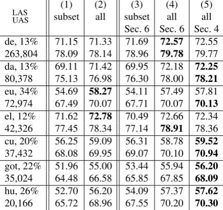
[image:12.595.72.290.58.263.2]UAS subset all subset all all Sec. 6 Sec. 6 Sec. 4 de, 13% 71.15 71.33 71.69 72.57 72.55 263,804 78.09 78.14 78.96 79.78 79.77 da, 13% 69.11 71.42 69.95 72.18 72.25 80,378 75.13 76.98 76.30 78.00 78.21 eu, 34% 54.69 58.27 54.11 57.49 57.81 72,974 67.49 70.07 67.71 70.07 70.13 el, 12% 71.62 72.78 70.49 72.66 72.34 42,326 77.45 78.34 77.14 78.91 78.36 cu, 20% 56.25 59.09 56.31 58.78 59.52 37,432 68.08 69.95 69.07 70.10 70.94 got, 22% 51.96 55.00 53.44 55.94 56.20 35,024 64.48 66.58 65.85 67.85 68.09 hu, 26% 52.70 56.20 54.09 57.37 57.62 20,166 65.72 68.96 67.55 70.20 70.30
Table 7: Accuracies, with percentage of trees that are non-projective, and number of tokens. Only gold computations are considered in a single pass (1,2) or there is a second pass as well (3,4,5). The first pass is on the subset of projective trees (1,3) or on all trees after optimal projectivization (2,4,5). The second pass is on projectivized trees (3,4) or on unprojectivized trees (5).
The main advantage of the cubic-time algorithm is that it is also applicable if the training corpus has not been projectivized. To explore this we have run this algorithm on the same corpus again, but now without projectivization in the second pass (for training the classifier in the first pass, projec-tivization was done as before). In this case, we can no longer remove non-critical nodes (without it affecting correctness), and now the curve is mono-tone increasing, as shown by Section 4 (unproj) in Figure 9. Nevertheless, with mean running times below 0.25 sec even for input longer than 100 tokens, this algorithm is practically relevant.
8.3 Accuracy
If a corpus is large enough for the parameters of a classifier to be reliably estimated, or if the vast majority of trees is projective, then accuracy is not likely to be much affected by the work in this paper. We therefore also consider six languages that have some of the smallest corpora in UD v2.2 in combination with a relatively large proportion of non-projective trees: Danish, Basque, Greek, Old Church Slanovic, Gothic, and Hungarian. For these languages, Table 7 shows that accuracy is generally higher if training can benefit from all
trees. In a few cases, it appears to be slightly better to train directly on non-projective trees rather than on optimally projectivized trees.
9 Conclusions
We have presented the first algorithm to calculate the optimal step for shift-reduce dependency pars-ing that is applicable on non-projective trainpars-ing corpora. Perhaps even more innovative than its functionality is its modular architecture, which im-plies that the same is possible for related kinds of parsing, as long as the set of allowable transitions can be described in terms of a split context-free grammar. The application of the framework to, among others, arc-eager dependency parsing is to be reported elsewhere.
We have also shown that calculation of the optimal step is possible in linear time if the train-ing corpus is projective. This is the first time this has been shown for a form of projective, deter-ministic dependency parsing that does not have the property of arc-decomposibility.
Acknowledgments
The author wishes to thank the reviewers for comments and suggestions, which led to substan-tial improvements.
References
Lauriane Aufrant, Guillaume Wisniewski, and Franc¸ois Yvon. 2018. Exploiting dynamic ora-cles to train projective dependency parsers on non-projective trees. In Conference of the North American Chapter of the Association for Computational Linguistics: Human Lan-guage Technologies, volume 2, pages 413–419. New Orleans, LA.
Jinho D. Choi and Martha Palmer. 2011. Getting the most out of transition-based dependency pars-ing. In49th Annual Meeting of the Association for Computational Linguistics, Proceedings of the Conference, pages 687–692. Portland, OR.
Jason Eisner and Giorgio Satta. 1999. Efficient parsing for bilexical context-free grammars and head automaton grammars. In37th Annual Meeting of the Association for Computational Linguistics, Proceedings of the Conference, pages 457–464. Maryland.
Daniel Fern´andez-Gonz´alez and Carlos G´omez-Rodr´ıguez. 2018a. A dynamic oracle for linear-time 2-planar dependency parsing. InConference of the North American Chapter of the Asso-ciation for Computational Linguistics: Human Lan-guage Technologies, volume 2, pages 386–392. New Orleans, LA.
Daniel Fern´andez-Gonz´alez and Carlos G´omez-Rodr´ıguez. 2018b. Non-projective dependency parsing with non-local transitions. In Con-ference of the North American Chapter of the Association for Computational Linguistics: Human Language Technologies, volume 2, pages 693–700. New Orleans, LA.
Norman Fraser. 1989. Parsing and dependency grammar.UCL Working Papers in Linguistics, 1:296–319.
Yoav Goldberg and Joakim Nivre. 2012. A dy-namic oracle for arc-eager dependency parsing. InThe 24th International Conference on Com-putational Linguistics, pages 959–976. Mumbai.
Yoav Goldberg and Joakim Nivre. 2013. Training deterministic parsers with non-deterministic oracles. Transactions of the Association for Computational Linguistics, 1:403–414.
Yoav Goldberg, Francesco Sartorio, and Giorgio Satta. 2014. A tabular method for dynamic ora-cles in transition-based parsing.Transactions of the Association for Computational Linguistics, 2:119–130.
Carlos G´omez-Rodr´ıguez, John Carroll, and David Weir. 2008. A deductive approach to depen-dency parsing. In 46th Annual Meeting of the Association for Computational Linguistics: Hu-man Language Technologies, pages 968–976. Columbus, OH.
Carlos G´omez-Rodr´ıguez and Daniel Fern´andez-Gonz´alez. 2015. An efficient dynamic oracle for unrestricted non-projective parsing. In53rd Annual Meeting of the Association for Compu-tational Linguistics and 7th International Joint
Conference on Natural Language Processing, volume 2, pages 256–261. Beijing.
Carlos G´omez-Rodr´ıguez, Francesco Sartorio, and Giorgio Satta. 2014. A polynomial-time dynamic oracle for non-projective dependency parsing. In Conference on Empirical Methods in Natural Language Processing, Proceedings of the Conference, pages 917–927. Doha.
Liang Huang and Kenji Sagae. 2010. Dynamic pro-gramming for linear-time incremental parsing. InProceedings of the 48th Annual Meeting of the Association for Computational Linguistics, pages 1077–1086. Uppsala.
Mark Johnson. 2007. Transforming projective bilexical dependency grammars into efficiently-parsable CFGs with Unfold-Fold. In 45th Annual Meeting of the Association for Com-putational Linguistics, Proceedings of the Con-ference, pages 168–175. Prague.
Sylvain Kahane, Alexis Nasr, and Owen Rambow. 1998. Pseudo-projectivity, a polynomially pars-able non-projective dependency grammar. In
36th Annual Meeting of the Association for Computational Linguistics and 17th Interna-tional Conference on ComputaInterna-tional Linguis-tics, volume 1, pages 646–652. Montreal.
Martin Kay. 2000. Guides and oracles for linear-time parsing. In Proceedings of the Sixth International Workshop on Parsing Technolo-gies, pages 6–9. Trento.
Marco Kuhlmann, Carlos G´omez-Rodr´ıguez, and Giorgio Satta. 2011. Dynamic programming algorithms for transition-based dependency pars-ers. In49th Annual Meeting of the Association for Computational Linguistics, Proceedings of the Conference, pages 673–682. Portland, OR.
Miryam de Lhoneux, Sara Stymne, and Joakim Nivre. 2017. Arc-hybrid non-projective depen-dency parsing with a static-dynamic oracle. In 15th International Conference on Parsing Technologies, pages 99–104. Pisa.
Joakim Nivre. 2008. Algorithms for deterministic incremental dependency parsing. Computa-tional Linguistics, 34(4):513–553.
Joakim Nivre, Johan Hall, and Jens Nilsson. 2004. Memory-based dependency parsing. In
Proceedings of the Eighth Conference on Computational Natural Language Learning, pages 49–56. Boston, MA.
Joakim Nivre and Jens Nilsson. 2005. Pseudo-projective dependency parsing. In43rd Annual Meeting of the Association for Computational Linguistics, Proceedings of the Conference, pages 99–106. Ann Arbor, MI.
Peng Qi and Christopher D. Manning. 2017. Arc-swift: A novel transition system for
depen-dency parsing. In 55th Annual Meeting of the Association for Computational Linguistics, Proceedings of the Conference, volume 2, pages 110–117. Vancouver.
Milan Straka, Jan Hajiˇc, Jana Strakov´a, and Jan Hajiˇc, jr. 2015. Parsing universal dependency treebanks using neural networks and search-based oracle. InProceedings of the Fourteenth International Workshop on Treebanks and Linguistic Theories, pages 208–220. Warsaw.