What are protoclusters? – Defining high-redshift galaxy clusters
and protoclusters
Stuart I. Muldrew,
1‹Nina A. Hatch
2and Elizabeth A. Cooke
21Department of Physics and Astronomy, University of Leicester, University Road, Leicester LE1 7RH, UK 2School of Physics and Astronomy, University of Nottingham, Nottingham NG7 2RD, UK
Accepted 2015 June 27. Received 2015 June 16; in original form 2015 March 16
A B S T R A C T
We explore the structures of protoclusters and their relationship with high-redshift clusters using the Millennium Simulation combined with a semi-analytic model. We find that proto-clusters are very extended, with 90 per cent of their mass spread across∼35h−1Mpc comoving atz=2 (∼30 arcmin). The ‘main halo’, which can manifest as a high-redshift cluster or group, is only a minor feature of the protocluster, containing less than 20 per cent of all protocluster galaxies atz=2. Furthermore, many protoclusters do not contain a main halo that is massive enough to be identified as a high-redshift cluster. Protoclusters exist in a range of evolutionary states at high redshift, independent of the mass they will evolve to atz=0. We show that the evolutionary state of a protocluster can be approximated by the mass ratio of the first and second most massive haloes within the protocluster, and thez=0 mass of a protocluster can be estimated to within 0.2 dex accuracy if both the mass of the main halo and the evolutionary state are known. We also investigate the biases introduced by only observing star-forming protocluster members within small fields. The star formation rate required for line-emitting galaxies to be detected is typically high, which leads to the artificial loss of low-mass galaxies from the protocluster sample. This effect is stronger for observations of the centre of the protocluster, where the quenched galaxy fraction is higher. This loss of low-mass galaxies, relative to the field, distorts the size of the galaxy overdensity, which in turn can contribute to errors in predicting thez=0 evolved mass.
Key words: methods: numerical – methods: statistical – galaxies: clusters: general – galaxies: evolution – galaxies: formation – cosmology: theory.
1 I N T R O D U C T I O N
In a cold dark matter universe with a cosmological constant (CDM), structure forms through hierarchical growth with smaller haloes merging to form larger ones. Galaxy clusters in the present day Universe are the most massive structures to have formed and were the result of the merging of many smaller haloes. Clusters, typically, are virialized dark matter haloes of mass greater than 1014M
containing a hot X-ray Intra-Cluster Medium (ICM) and red, passive galaxies.
At higher redshift,z >1.5, most clusters were not the massive virialized haloes that we see today. Instead we see their progeni-tors, a diffuse collection of haloes that will merge to make the final halo. The term ‘protocluster’ is often used to describe this state, but differing definitions of what a protocluster is exist in the literature. While some define a protocluster as all the haloes at a given redshift
E-mail:[email protected]
that will merge to make the final cluster, others define it as being just the most massive progenitor halo, sometimes referred to as the main halo. While using the latter definition dramatically reduces the observational expense, it risks missing galaxies undergoing en-vironmental preprocessing and only captures part of what is going on in the forming cluster.
Several high-redshift galaxy clusters have now been detected through X-ray emission, the Sunyaev–Zel’dovich (SZ) effect, as well as through photometric redshift hunts in large deep surveys (Gobat et al. 2011; Stanford et al. 2012; Zeimann et al. 2012; Fassbender et al.2014; Andreon et al. 2014). The properties of the ICM and galaxies indicate that these structures are already col-lapsed, i.e. these objects are single collapsed main haloes. How-ever, a great deal of cluster growth occurs at relatively late times (z >1; Chiang, Overzier & Gebhardt2013), and many of the galax-ies and dark matter that end up in thez= 0 cluster will not be located in the main halo of the protocluster at high redshift. In this paper we investigate how much of the matter and galaxies reside in the main halo compared to the entire protocluster as a function of
2015 The Authors
at University of Nottingham on July 7, 2016
http://mnras.oxfordjournals.org/
redshift, and use this to investigate its significance. Additionally, we look at whether protoclusters with evolved main haloes are rep-resentative of all protoclusters, or are a subsample that are easier to detect.
Identifying protoclusters has so far been challenging due to their low number density and the faintness of distant galaxies. One of the most successful methods for detecting protoclusters is to use High Redshift Radio Galaxies (HzRGs) as a tracer population to locate overdense regions (e.g. Le Fevre et al.1996; Pentericci et al.2000; Best et al.2003; Venemans et al.2007; Galametz et al.2010,2013; Hatch et al.2011a; Wylezalek et al.2013; Cooke et al.2014). These galaxies are among the most massive galaxies at all epochs (Sey-mour et al.2007), but the large galaxy overdensities that surround these radio-loud galaxies exceed that of similar mass radio-quiet galaxies (Hatch et al.2014). Both Ramos Almeida et al. (2013) and Hatch et al. (2014) concluded that dense environments foster the formation of radio-loud jets from AGN, which explains why HzRGs are excellent beacons of galaxy protoclusters and high-redshift clus-ters.
An alternative technique is to identify protoclusters in large sur-veys with accurate photometric redshifts. Precise photometric red-shifts atz≥2 are difficult to obtain due to the Balmer break shift-ing into the near-infrared wavelength, but Spitler et al. (2012) have shown that Virgo-like cluster progenitors can be found if medium-band near-infrared filters are used. Chiang et al. (2013) advocate a protocluster detection method that finds galaxy overdensities in 15 Mpc comoving windows; applying this method to the 1.62 deg2
COSMOS/UltraVISTA field (Muzzin et al.2013) has resulted in 36 candidate structures (Chiang, Overzier & Gebhardt2014). This method is effective because of the correlation between aperture density and halo mass (Haas, Schaye & Jeeson-Daniel2012; Mul-drew et al.2012); however at high redshift there is considerable uncertainty in this relation due to projection effects (Shattow et al.
2013).
A number of techniques have been used to isolate the galax-ies within high-redshift clusters and protoclusters for further study. Photometric redshifts from deep multi-band data can reach accura-cies ofz/(1+z)=0.03, and although (proto-)cluster galaxies have been selected using photometric redshifts (e.g. Tanaka et al.
2010), the sample is often incomplete and greatly contaminated by foreground and background galaxies. One of the most successful techniques for locating clean samples of protocluster galaxies is us-ing narrow-band filters with specific central wavelengths matched to the wavelength of an emission line from protocluster galaxies (e.g. Kurk et al.2004; Venemans et al.2007; Hatch et al.2011b; Cooke et al.2014). The ideal line is Hαsince it is a strong line which is least affected by dust absorption. Selecting galaxies based on their line emission means only active galaxies are located, i.e. star-forming galaxies and AGN. This can limit our view of the pro-tocluster in unexpected ways. Here we explore how this selection method can give a biased view of the protocluster.
In this paper we explore the galaxies that make up protoclusters using a semi-analytic model built upon the Millennium Simulation. In Section 2 we describe the simulations used and how we con-structed the protocluster catalogue. Using this mock catalogue, in Section 3, we give an overview of the spatial properties of protoclus-ters and their member galaxies. We then examine two fundamental issues concerning protoclusters: the relationship of the main progen-itor halo (which is sometimes observed as the high-redshift cluster) to the rest of the protocluster and the cluster’sz =0 mass; and how our understanding of protoclusters is biased when only active protocluster galaxies are observed. In Section 4 we summarize our
findings and reflect on the implications they have for interpreting observations of protoclusters and high-redshift clusters.
2 M E T H O D S
To construct a statistically large sample of galaxy clusters, whose evolution can be tracked back to high redshift, we used the Guo et al. (2011) semi-analytic model applied to the Millennium Simulation (Springel et al.2005). Clusters were identified as haloes with masses greater than 1014h−1M
atz=0, while protoclusters were defined as the cluster progenitors.
2.1 The Millennium Simulation and semi-analytic model
The Millennium Simulation follows the evolution of 21603 dark
matter particles in a cube of comoving side length 500h−1Mpc,
using theN-body codeGADGET-2 (Springel2005). It adopts aCDM
cosmology with parameters0=0.25,=0.75,h=0.73,n=1
andσ8=0.9 consistent with the Two-Degree Field Galaxy Redshift
Survey (2dFGRS; Colless et al.2001) and the first-yearWilkinson Microwave Anisotropy Probedata (WMAP-1; Spergel et al.2003). Haloes were detected using a two-step procedure. First, a Friends-of-Friends algorithm (FoF; Davis et al.1985) with linking length,
b= 0.2, was used to identify haloes and these were then post-processed using SUBFIND (Springel et al. 2001). All haloes with greater than 20 particles were used to construct merger trees. We note similar results are found with other halo finders (Muldrew, Pearce & Power2011; Knebe et al.2011).
To populate the simulation with galaxies, the Guo et al. (2011) semi-analytic model was applied to the resulting merger trees. This model is an updated version of that previously presented in Croton et al. (2006) and De Lucia & Blaizot (2007) and gives a better fit to the redshift evolution in the galaxy stellar mass function. The model includes prescriptions for gas infall, shock heating, cooling, star formation, stellar evolution, supernova feedback, black hole growth and feedback, metal enrichment, mergers, and tidal and ram-pressure stripping. Full details of these implementations can be found within the previously referenced papers. For the purpose of this study we cut the semi-analytic catalogue to only include galaxies with stellar masses greater than 108h−1M
. This is above the resolution limit adopted by Guo et al. (2011), but is still below the detection threshold of most observational protocluster studies (e.g. Cooke et al.2014). All results that are dependent on stellar mass in this paper are presented against mass or with different minimum cuts to illustrate the effect of having a minimum galaxy mass cut.
The cosmological parameters used for the Millennium Simulation were in agreement with the results ofWMAP-1, but have become slightly discrepant with the latest values fromPlanck(Planck Col-laboration I et al.2014). Angulo & White (2010) proposed a method of rescaling dark matter simulations to different cosmologies by re-assigning the mass and position of particles and the redshift of the snapshot. Guo et al. (2013) applied this method to the Millennium Simulation to obtain a galaxy catalogue forWMAP-7 cosmology (Komatsu et al.2011). They found that the increased matter density, m, offsets the effect of a decreased linear fluctuation amplitude,σ8,
which leads to very similar results forz <3. This should have even less of an effect forPlanckcosmology, where the rescaling from
WMAP-1 is not as large (Henriques et al.2015). Further comparison for protoclusters betweenWMAP-1 andWMAP-7 cosmology was made by Chiang et al. (2013), who found little difference in results.
at University of Nottingham on July 7, 2016
http://mnras.oxfordjournals.org/
This confirms that using a simulation based onWMAP-1 cosmology will have little overall impact on our results.
2.2 Protocluster identification
We identified galaxy clusters in the simulation exclusively on dark matter halo mass. All haloes with M200 ≥ 1014h−1M at z =
0, where M200 is the mass enclosed by a sphere whose density
is 200 times the critical density of the Universe, were defined as galaxy clusters. This gave a total of 1938 clusters in our sample. All semi-analytic galaxies that are members of the FoF haloes are then classed as galaxy cluster members. Each halo consists of a ‘central’ galaxy, which is at the centre of the halo, and ‘satellite’ galaxies.
For protoclusters, we trace the merger tree back in time to each redshift of interest. For eachz=0 cluster, we identify all the haloes at a given redshift that will merge to form it and identify this as the protocluster. All galaxies that are associated with these haloes are then classed as protocluster members. For example, atz=2 there are 1938 protoclusters, which are the progenitors of the z =0 clusters, but these are made up of 639 253 individual haloes with a central galaxy of at leastM∗=108h−1M
. Unless stated otherwise, the protocluster studies presented in this paper are forz =2.
3 R E S U LT S
The results are presented in three sections looking at different as-pects of protoclusters. First in Section 3.1 we explore the distribu-tion of protocluster member galaxies to explain what protoclusters are. In Section 3.2 we examine the relationship between protoclus-ters and their main haloes. Finally, in Section 3.3 we explore how limiting our observations to only the active subset of protocluster galaxies can affect our understanding of protoclusters.
3.1 The distribution of protocluster galaxies
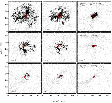
To begin, we explore the distribution of galaxies that make up a protocluster. Fig.1displays the spatial extent of protocluster galaxy members, with mass M∗ ≥ 108h−1M
at z = 2, 1 and 0 for Mz=0
200 masses of 1014.0, 1014.8 and 1015.4h−1M. The red circle
corresponds to the comovingz=0 virial radius of the cluster. At z=2 theM200z=0=1015.4h−1Mcluster (top left panel) extends
to 45h−1Mpc comoving (15h−1Mpc physical), showing a rich
structure of haloes and filaments. The structure is far from the collapsed single halo it becomes atz=0 (top right panel). For the lower mass clusters, a similar filamentary distribution is visible at high redshift, but the overall spread is much smaller.
Due to the limit of instrumental fields-of-view, targeted observa-tional imaging studies of protoclusters have typical windows of a few arcmin on a side (e.g. 2.5 arcmin in Cooke et al.2014or 7 arcmin in Koyama et al.2013). Forz=2, and the cosmology of the Millen-nium Simulation, this corresponds to 2.8h−1Mpc and 7.7h−1Mpc
comoving, respectively (determined using ‘The Cosmology Calcu-lator’; Wright2006). Comparing these to the full distribution of the protocluster, the left-hand panels of Fig.1demonstrate that in all but the lowest mass case, only a small area of the protocluster is being captured. In the top panel, for the most massive cluster, the red circle corresponds to thez=0 virial radius of 2.16h−1Mpc
comoving. This circle would enclose the smaller aperture of Cooke et al. (2014). This means that any observations of protoclusters car-ried out in this way are not following the entire protocluster, but are focused on just the growth of the central region.
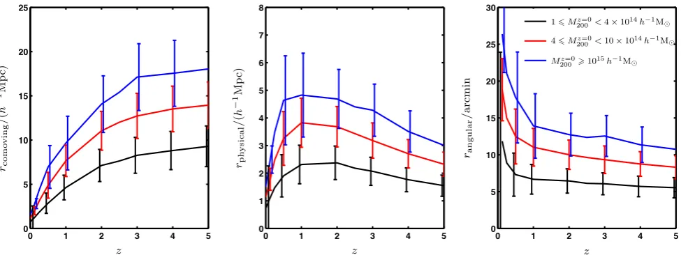
To further illustrate the large spatial extent of the protocluster, we plot the radius that encloses 90 per cent of the stellar mass at different redshifts in Fig.2. The 90 per cent stellar mass radius is strongly correlated to the 90 per cent dark matter mass radius, making it an excellent measure of cosmological growth. The proto-clusters are binned by theirz=0 mass and sizes are presented in comoving, physical and angular scale. We explore the difference be-tween defining cluster members using the FoF halo or virial radius in the Appendix.
In the comoving reference frame, protoclusters continually col-lapse, albeit gradually abovez =3. At these high redshifts, the protoclusters display a similar comoving size, for fixedz=0 mass, indicative of the shorter amount of cosmic time that passes com-pared to lower redshift and the late collapse of clusters. The dif-ference in size with mass at fixed redshift is also much larger at high redshift compared with the present day. The large sizes are in agreement with those found by Chiang et al. (2013) using an alternative measure of the protocluster’s radius.
In physical units, the behaviour of the protocluster appears quite different. At high redshift protoclusters are still expanding with the Universe before collapse occurs afterz = 1. Therefore the global density of protoclusters decreases with time untilz∼1, after which they rapidly collapse. From an observational point of view, protoclusters extend over approximately the same angle across the sky fromz∼5 toz∼1. This means that protocluster detection algorithms do not need to search over different-sized apertures to locate protoclusters at different redshifts: a single fixed angular aperture will suffice. However the size of the aperture could be adjusted to select different mass protoclusters. Additionally, the large spatial extent of protoclusters means that using off-centre galaxies as a field sample may not produce a clean sample. As emphasized in Fig.1, the complex structure of protoclusters means they can be very extended in one direction. Therefore, even at large radii from the protocluster core there may be dense regions of protocluster galaxies. To be certain of having a clean field sample for comparisons, field galaxies should be selected from regions more than 20 arcmin from the protocluster core. This conclusion correlates with low-redshift theoretical and observational studies of clusters that have also emphasized the importance of selecting field samples far away from the cluster (e.g. Bah´e et al.2013; Haines et al.2015).
The next generation of large galaxy surveys, such as the Large Synoptic Survey Telescope (LSST) andEuclid, have the potential to locate many protoclusters and high-redshift clusters. Existing tech-niques used to detect clusters at low redshift, such as X-ray identifi-cation or using the red sequence, are not suitable for protoclusters as they are not evolved enough to possess these properties. However, one method of detecting protoclusters that would be suitable is to use an environment measure to identify overdensities. In Fig.3we plot the third nearest-neighbour density against galaxy stellar mass for all galaxies in the Millennium Simulation and those we have defined as protocluster members (any galaxy that will merge into thez=0 clusters). The environment is characterized usingδ:
δ= ρ−ρ¯ ¯
ρ =
ρ ¯
ρ −1, (1)
whereρ is the galaxy density and ¯ρis the average density of all galaxies. As expected, there is a clear trend for massive galaxies to reside in denser environments. For very massive galaxies there is little difference between the environments occupied by protocluster galaxies and all galaxies. This implies that most massive galaxies at high redshift reside in protoclusters. For lower mass galaxies, the
at University of Nottingham on July 7, 2016
http://mnras.oxfordjournals.org/
Figure 1. The spatial extent of protoclusters atz=2 (left panel), 1 (centre panel) and 0 (right panel), with final cluster masses ofM200z=0=1015.4h−1M (top row), 1014.8h−1M
(middle row) and 1014.0h−1M
(bottom row). Each window is 45×45h−1Mpc comoving, which corresponds to 41 arcmin and 65 arcmin atz=2 andz=1, respectively (Wright2006). Black points represent a galaxy of stellar mass greater than 108h−1M
that will end up in the cluster while grey points represent those that will not. (Only 25 per cent of the background galaxies, grey points, are plotted to reduce image size.) The red circle corresponds to thez=0 centre and comoving viral radius of the cluster.
Figure 2. The average radius that encloses 90 per cent of the stellar mass of a protocluster at different redshifts, for binnedz=0 cluster masses. The left panel represents comoving radius, centre panel the physical radius and right panel the angular projection. Error bars represent 1σscatter and are offset about the middle mass bin byδz=0.05 for clarity. This radius is tightly correlated with the radius enclosing 90 per cent of the dark matter mass.
two curves diverge showing that the third nearest-neighbour den-sity measure can pick out the protocluster overdenden-sity relative to the field for all masses. This means that measuring the environment of low-mass galaxies around high-mass galaxies offers the oppor-tunity to locate protoclusters in large photometric redshift surveys.
Measuring accurate environments is more difficult at high redshift (Shattow et al.2013) and the ability to accurately detect protoclus-ters using this method will be explored in future work.
Finally, we look at the level of contamination associated with the size of the aperture. As we have seen, the limitations due to
at University of Nottingham on July 7, 2016
http://mnras.oxfordjournals.org/
[image:4.595.51.546.478.628.2]Figure 3. The third nearest-neighbour galaxy density of protocluster galax-ies (red dashed line) relative to all galaxgalax-ies (solid black line), as a function of stellar mass. High-mass galaxies show similar environments due to most of them being in protoclusters; however low-mass galaxies diverge.
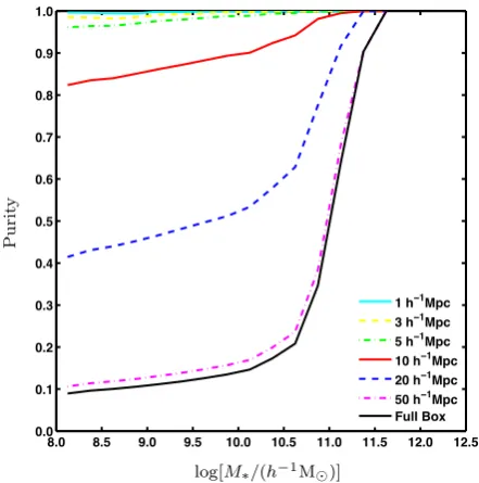
Figure 4. The fraction ofz=2 galaxies within a given comoving volume, centred on the largest protocluster halo, that are protocluster members. Apertures are defined as the side length of a cube. Small apertures that are typical of Hαnarrow-band imaging produce low contamination.
instrumental fields-of-view mean that we are limited to small aper-tures which do not capture the full protocluster. Using a larger aperture would capture the whole protocluster, but would introduce a higher level of contamination from non-protocluster members.
[image:5.595.51.277.57.282.2]In Fig. 4 we plot the fraction of galaxies that are protoclus-ter members for different masses within different-sized apertures. Apertures are defined as the side length of a cube. For all apertures there is little contamination at the very high mass end reaffirming our conclusion that most high-mass galaxies are in protoclusters. This also reaffirms the previous conclusion that in order to attain a
Figure 5. The evolution of halo mass for clusters binned byz=0 mass. The lines show the fraction of mass in the main halo (solid line) and all haloes that will merge to make the final cluster (dashed line) relative to thez=0 mass of the halo for differentz=0 mass clusters. Most of the protocluster mass is spread amongst many haloes and not concentrated in the main halo. Error bars represent 1σscatter and are offset about the middle mass bin by
δz=0.05 for clarity.
clean sample of field galaxies it is important to search further than 20 arcmin from the protocluster, as many galaxies, especially those withM∗>1010.5M
, closer than this are likely to be protocluster members. For small apertures the level of contamination is low at all masses, reflecting the fact that only a small amount of the proto-cluster is being detected. For large apertures, the contamination is significant for low-mass galaxies and by 50h−1Mpc it is the same
as randomly sampling the Universe. This implies that small aper-tures (<10h−1Mpc) are required to produce a clean sample. If the
protocluster galaxies are defined as all those that enter the virial radius byz=0, all of these purity fractions decrease by approxi-mately a few to 10 per cent. Furthermore, the contamination levels presented here are lower limits due to the use of cubes. In reality, thezdimension would be significantly larger than the other two dimensions, in most cases, due to redshift uncertainties. This would increase the level of contamination.
3.2 The relationship between a protocluster and its main halo
In Fig.1we showed that the protocluster environment is a complex ‘clumpy’ structure. We define the main halo as being the most massive progenitor halo in the protocluster at a given redshift. If the main halo is massive enough it will be observed as a high-redshift cluster.
3.2.1 Main halo versus protocluster mass
To explore how the growth of the main halo relates to the proto-cluster as a whole, in Fig.5we plot the mass assembly of both. The solid lines correspond to the fraction of thez=0 halo mass that is present in the largest progenitor halo with redshift. The dashed lines correspond to the fraction of mass in all haloes hosting a galaxy of at leastM∗=108h−1M
, at that redshift, that will merge to form
at University of Nottingham on July 7, 2016
http://mnras.oxfordjournals.org/
[image:5.595.52.273.341.564.2]Figure 6. The fraction of galaxies in the main halo compared to the full protocluster with redshift. Solid lines are for galaxies with stellar massM∗
>109h−1M
, while dashed lines are forM∗>1010h−1M
. Colours correspond to different cluster masses binned byz=0 mass. Galaxies of higher mass are more likely to be found in the main halo.
the final cluster. The assembly plot has been grouped by final mass and, as expected from hierarchical growth, high-mass clusters build up their mass later, although this is within the 1σerror.
The rate of mass growth of the main halo differs from that of the whole protocluster. The growth of the main halo is slower than the rest of the haloes in the protocluster atz >2, but atz <2 the main halo grows more rapidly. This is a manifestation of the hierarchical growth of dark matter structures. In the early Universe there is a rapid increase in the number of small dark matter haloes in the protocluster that become large enough to host a galaxy. Also, at low redshift (z <0.5), there are significantly fewer dark matter haloes remaining in the protocluster which have not yet merged with the main halo.
Fig.5illustrates that less than∼20 per cent of the protoclusters mass is in the main halo at high redshift (z >2). Forz=2 the main halo contains only∼10 per cent of thez=0 cluster’s mass for a massive halo. This means that studying only the main progenitor ignores a vast amount of information about the forming cluster.
Fig.5considered the growth of the dark matter halo. We now look at the galaxies that reside in the main halo compared to the protocluster by plotting the fraction of galaxies in the main halo in Fig.6. These fractions are determined using two different stellar mass cuts. As the redshift decreases the fraction of protocluster galaxies in the main halo increases forM∗>109h−1M. This is
expected as merging with the main halo brings galaxies that were residing outside of it in.
For a higher stellar mass cut ofM∗ >1010h−1M
, however, there is an unexpectedly different trend. As the redshift decreases toz=3, the fraction of galaxies in the main halo decreases before increasing again after this point. Massive galaxies cannot leave the main halo, therefore this effect can only occur by galaxies outside of the main halo gaining enough mass to enter the sample. These trends are apparent for all mass protoclusters. Additionally, the most massive halo of higher mass protoclusters is less significant as it hosts a smaller fraction of the total galaxies.
Regardless of cluster mass, no main halo hosts more than 30 per cent of protocluster galaxies with M∗ > 109h−1M
at z >2. Observations that only study galaxies within the main pro-genitor halo (i.e. the high-redshift cluster) miss the majority of cluster galaxy progenitors. To trace the evolution of cluster galax-ies, it is essential that a representative fraction of the protocluster is observed.
3.2.2 Estimating thez=0 cluster mass from the main halo mass at high redshift
Having shown that the main halo contains only a fraction of the mass and galaxies of the protocluster, we now explore how much the structure of the protocluster can reveal about its evolutionary state, and the mass of the cluster it will become byz=0. The evolutionary state of a protocluster is described by the fraction of matter already located within the main protocluster halo. Protoclusters that contain a high fraction of their mass within the main halo are defined as further evolved.
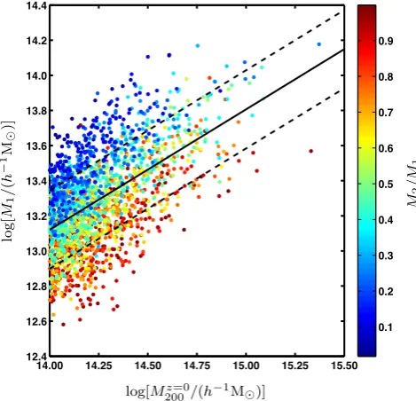
Fig.7plots the mass of the main halo atz=2 against the mass of the cluster atz=0. The median best fit to the data and 1σdeviation are shown by the black solid and dashed lines. These are determined by bootstrap sampling 100 000 times the least-squares fit. There is a clear correlation between the mass of the main progenitor halo at z=2 and the mass of the resultantz=0 cluster: more massive progenitors tend to evolve into more massive clusters. However, for a givenz=0 cluster mass, there is a large scatter in the range of masses for the main halo of the protocluster atz=2. This means that protoclusters exist in a range of evolutionary states at high red-shift, which is nearly independent of the mass they will grow to by z=0. Thus estimating thez=0 mass of a cluster by extrapolating the mass of the high-redshift cluster should be considered highly uncertain due to variation in the accretion history during cluster formation.
If more than one progenitor halo can be identified, and its mass measured, the accuracy and precision of the extrapolation will in-crease. Each point in Fig.7is colour coded to indicate the ratio of the mass of the second most massive halo in the protocluster (M2) to
the most massive (M1) atz=2, i.e. an indication of the dominance
of the main halo in the protocluster. Clusters of all mass have a huge range in this ratio at higher redshift indicating the stochastic nature of cluster formation. The scatter in the relation between the cluster’s mass atz= 2 andz =0 separates into clear bands of protoclusters at different evolutionary states at that redshift. There-fore the mass ratio of the two most massive protocluster haloes (M1andM2) provides an approximation of the evolutionary state of
the protocluster.
Fig.8shows two of these bands: protoclusters with dominant main haloes (blue points;M2/M1<0.15) and protoclusters in which
there is no single dominant halo (red points;M2/M1>0.85). The
solid lines represent the median best fit to these data, with dashed lines showing the 1σ scatter about these lines. Both are again ob-tained by bootstrap sampling 100 000 times the least-squares fit. Clusters with a single, dominant progenitor halo (blue points) tend to have largerz=2 masses than those with higherM2/M1ratios
(red points) and correlate more strongly withz=0 cluster mass. Extrapolating the main halo mass to the z= 0 cluster mass, whilst taking into account the mass ratio of the two most massive haloes within the protocluster, will not only improve the preci-sion but also the accuracy. For protoclusters withM2/M1<0.15,
the scatter in the mass of the main halo at z = 2 for a given
at University of Nottingham on July 7, 2016
http://mnras.oxfordjournals.org/
[image:6.595.56.277.56.273.2]Figure 7. The mass of the most massive progenitor halo (M1) atz=2 for a givenz=0 cluster mass. Points are coloured by the ratio of the mass of second most massive progenitor (M2) to the first most massive (M1) at z=2. The solid black line gives the best fit to the data with dashed lines representing the 1σscatter about this.
z=0 cluster mass halves. Additionally, the accuracy of this mea-surement increases, which can be quantified by considering the RMS of the difference between the predicted and truez=0 mass cluster. For protoclusters withM2/M1<0.15, the estimate of the
z=0 mass made without any information about theM2/M1ratio
(i.e. using the black dot–dashed fit) would have a 0.54 dex RMS deviation from the true mass; however this decreases to 0.15 dex when the ratio is taken into account (using the blue fit). Observa-tional studies that wish to estimate thez=0 mass of a protocluster may therefore improve the accuracy and precision of their esti-mate by measuring the mass of the two most massive haloes in the protocluster.
The masses of the two most massive haloes within a protocluster can be measured observationally in a number of ways. Galaxy ve-locity dispersions can give an estimate of the dynamical mass under the assumption that the galaxies are in virial equilibrium. Such a method has been used by Shimakawa et al. (2014) to estimate the mass of two groups in az=2.53 protocluster, finding a ratio of ∼0.1. Alternatively, the mass of the haloes can be measured through observations of the intracluster gas using sensitive X-ray observa-tories, or at submillimetre wavelengths to detect the SZ decrement. Current instrumentation is only able to measure collapsed structures atz >1.5 with masses greater than 1013.7M
(e.g. Brodwin et al.
2012; Stanford et al.2012; Andreon et al. 2014), but forthcom-ing instrumentation, such as the ESAAthenasatellite and the full ALMA array, will be able to detect much smaller groups at high redshift. If the ratio ofM2/M1is sufficiently small, then it may not
be possible to measure the mass ofM2directly through X-rays or
the SZ decrement. In this case, it may be sufficient to measure the mass ofM1through a detection of the ICM and estimate the mass
ofM2through the ratio of stellar mass enclosed inM2andM1. The
stellar mass is a good tracer of the total cluster mass at low and intermediate redshifts (Mulroy et al.2014; Ziparo et al., in prepara-tion) and the next generation of accurate cosmological simulations
Figure 8. Same as Fig.7, but this time only protoclusters with a mass ratio of the second most massive progenitor to the first most massive (M2/M1), atz=2, greater than 0.85 (red) and less than 0.15 (blue) are shown. The solid lines give the best fit to the data with dashed lines representing the 1σ scatter about this. The black dot–dashed line represents the fit to allM2/M1 values.
will help determine the relationship between the stellar mass and the total mass within more distant groups.
3.2.3 The importance of the main halo within a protocluster
We further explore the scatter in cluster formation history by show-ing the fraction of protoclusters where the mass ratio of the second to the first most massive halo is more than a given value. The left panel of Fig.9shows that the second most massive halo is at least 80 per cent of the mass of the most massive halo in∼20 per cent of protoclusters. Only 10 per cent of protoclusters have a dominant main halo where the next largest is less than 20 per cent. These results are independent of thez= 0 mass of the cluster except in the largest mass bin where there are few objects, which means the accretion history of clusters is erratic for clusters of all mass. The right panel of Fig.9shows the same mass ratios, but this time against the mass of the main halo atz=2. A clear mass dependence can be seen with large main haloes significantly less likely to have a massive companion in the protocluster.
Overall, these figures illustrate that the largest halo in many pro-toclusters should not be considered the dominant halo as it is often not significantly larger than other haloes. These results also suggest that the observed examples of main halo dominated protoclusters is the result of potential bias in the observations. Larger main haloes are easier to detect using current cluster-finding techniques (e.g. red sequence algorithms, X-ray or SZ detections). Since it is eas-ier to locate high-redshift clusters with massive first ranked haloes, this subsample of evolved protoclusters will dominate observations. However, a significant fraction of massive clusters atz=0 do not yet have massive dominant haloes during the protocluster stage at high redshift. These less-evolved cluster progenitors would be missed by surveys searching for high-redshift clusters, which target
at University of Nottingham on July 7, 2016
http://mnras.oxfordjournals.org/
[image:7.595.44.279.57.283.2]Figure 9. The fraction of protoclusters atz=2 where the second most massive halo is greater than 0.8 (black solid), 0.6 (red dashed), 0.4 (blue dot–dashed) or 0.2 (magenta solid) times the mass of the most massive halo. The left panel presents this against thez=0 cluster mass while the right panel is against the most massive halo in the protocluster.
the most massive objects, and yet, they are equally likely to evolve into massive clusters byz=0. It is possible that the accretion his-tory of a cluster leaves a lasting trace on its gas properties and the distribution of its galaxies. To trace the different evolutionary paths taken by collapsing clusters we must search for all types of cluster progenitors.
If the whole of the protocluster cannot be viewed, and it is not clear if there is a main halo, it is important to see if the choice of the image centre has an effect on the results obtained. For protoclusters selected due to the presence of a radio-loud AGN (such as the Clusters Around Radio-Loud AGN (CARLA) Survey; Wylezalek et al.2013), often the centre of the protocluster is assumed to be the position of the radio-loud AGN, which is typically one of the most massive galaxies in the protocluster.
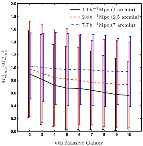
In Fig.10we present the stellar mass enclosed by various sized apertures, centred on the 10 most massive galaxies in the proto-cluster atz=2, with respect to that centred on the most massive. For an aperture of 7.7h−1Mpc (7 arcmin) the difference in enclosed
mass between an aperture centred on the first and 10th most massive galaxy is small, dropping to 94 per cent of the first most massive. For the smallest aperture tested of 1.1h−1Mpc (1 arcmin), however,
the drop is significantly larger, decreasing to 56 per cent mass of the one centred on the most massive galaxy. An analogous calculation can be made for enclosed star formation rate which shows a smaller change.
The most noticeable part of Fig.10is the huge scatter between protoclusters. For the smallest aperture tested, the mass enclosed by an aperture centred on the 10th most massive galaxy can vary from a decrease by a factor of 0.03 to an increase by a factor of 5 on that of an aperture centred on the most massive galaxy. This large variation means there is a large uncertainty associated with the observed mass and star formation rate of protoclusters if the main halo cannot be readily identified. Observing large sam-ples of protoclusters removes much of this uncertainty; therefore large statistical studies of protoclusters are less affected by this issue.
Figure 10. The effect of centring on the stellar mass enclosed in a cubical aperture of side length 1.1h−1Mpc (solid line), 2.8h−1Mpc (dashed) and 7.7h−1Mpc (dot–dashed). Each curve gives the total stellar mass enclosed when thenth most massive galaxy in the protocluster is chosen as the centre with respect to the most massive. For large apertures the difference in stellar mass is small; however the scatter between protoclusters is large. Error bars represent the 1σscatter and are offset for clarity.
3.3 Biases introduced by observing only star-forming protocluster galaxies
A very common technique to locate a clean sample of protoclus-ter galaxies is to select line-emitting galaxies, such as Hα, Lyα and [OII] emitters, using narrow filters (e.g. Venemans et al.2007;
at University of Nottingham on July 7, 2016
http://mnras.oxfordjournals.org/
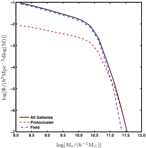
[image:8.595.308.550.334.581.2]Figure 11. The galaxy stellar mass function for all galaxies within the simulation atz=2 (black solid line), those tagged as protocluster galaxies (red dashed line) and those tagged as field galaxies (i.e. not protoclusters; blue dot–dashed line). The protocluster mass function has more massive galaxies and a shallower low-mass slope.
Koyama et al.2013). However, this method is only able to identify the active subset of protocluster galaxies. Here we explore how our interpretation of the galaxy stellar mass function and overdensity of the protocluster can be affected by only studying the star-forming galaxy population.
In Fig.11we plot the galaxy stellar mass function for protocluster members (red dashed line), field galaxies (non-protocluster mem-bers; blue dot–dashed line) and all galaxies (the sum of the two; black solid line) atz=2. The shape of the protocluster mass func-tion compared to the field differs slightly. There are more massive galaxies in protoclusters than the field, despite there being more galaxies in general in the field. At the low-mass end, the slope of the protocluster mass function is shallower than that of the field. The value for the turnover (M∗) is fractionally higher for the pro-tocluster. The shallower low-mass slope in the semi-analytic model protoclusters reduces the number of expected low-mass galaxies compared to the field, but not greatly.
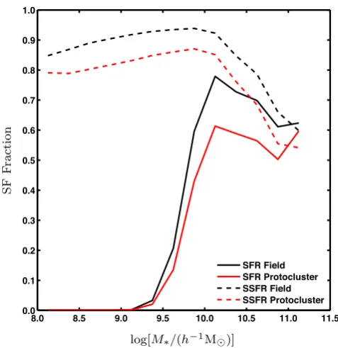
Conventional definitions of star-forming and non-star-forming galaxies involve cuts in Specific Star Formation Rate (sSFR; SFR/M∗). One such definition, used in Lani et al. (2013) for exam-ple, is to define a galaxy as non-star-forming if its mass doubling time, calculated from its present star formation rate, is more than the age of the Universe. Applying this to our simulatedz=2 galaxy sample yields a star-forming galaxy fraction corresponding to the dashed line in Fig.12. This demonstrates that there are fewer star-forming galaxies in the protocluster than the field, but in general they follow the same trend with mass.
Imaging in a narrow-band to detect emission line galaxies does not select galaxies based on their sSFR, but instead produces a cut in SFR. This can have a different effect, especially at the low-mass end, as a galaxy’s SFR is dependent on its mass if it is on the main star-forming sequence. Applying a cut of 7 Myr−1 (typical of
recent works; e.g. Cooke et al.2014) gives a star-forming fraction
that corresponds to the solid lines in Fig.12. This produces very different trend to that of the sSFR cut. At low masses, the star-forming fraction rapidly descends to zero as the cut intercepts the star-forming main sequence. This leads to a minimum detectable mass for emission-line-selected galaxies such as those observed in Hαnarrow-band images. Thus selecting galaxies by their star formation rate biases against low-mass galaxies.
The limitations of instrumental field of view mean that only a small fraction of the protocluster is typically observed. If we consider only the central region of the protocluster, rather than all members, we get a further bias in the results. Fig.13replots the star-forming fraction of protocluster and field galaxies with a 7 Myr−1
cut (solid lines), but only including the star-forming galaxies within the central 2.8h−1Mpc comoving (2.5 arcmin; blue dashed line) and
1.1h−1Mpc comoving (1 arcmin; blue dot–dashed line) regions of
the protocluster. Using the small window only captures the densest region where quenching is efficient and has led to a much lower fraction of star-forming galaxies relative to the field.
By observing only the star-forming galaxies in the main halo of the protocluster we obtain a very biased view of the mass function of protocluster galaxies. Having a fixed threshold intercepts the star-forming main sequence resulting in the suppression of galax-ies detected below 1010M
and a near total loss of galaxies be-low 109M
. In addition to the loss of galaxies because they drop below the star formation rate threshold, the small windows used for narrow-band observations result in a further loss. Focusing on just the very centre, as opposed to the full protocluster, signifi-cantly increases the quenched fraction of galaxies. This is because more environmental quenching occurs within the densest part of the protocluster. While larger apertures would reveal more of the protocluster, it would also increase the level of contamination of non-protocluster members. For small apertures the sample has little contamination, but by 10h−1Mpc at least 20 per cent of low-mass
galaxies are interlopers.
An important side effect of losing low-mass galaxies in narrow-band observations is that the measured overdensities for protocluster will be highly uncertain. If the full observed sample of galaxies is used, then the absence of low-mass galaxies in the protocluster compared with the field will lead to the overdensity being under-estimated. Using a mass cut, however, is also problematic. The simulations indicate that almost all very massive galaxies reside in protoclusters and this will lead to an unrepresentative field sample, leading to a very high overdensity estimate. Quantifying the over-density accurately is important for estimating the eventual mass of the protocluster using the Chiang et al. (2013) method. Due to the above reasons, it is not advisable to estimate the mass of a proto-cluster from the overdensity measured from the excess of emission line galaxies in a small field of view.
4 I M P L I C AT I O N S F O R O B S E RVAT I O N S
We have explored the difference between protoclusters and high-redshift clusters using a semi-analytic model applied to the Mil-lennium Simulation. Clusters were identified asz=0 haloes with masses greater than or equal to 1014h−1M
. All galaxies that will merge to make these clusters were tagged at higher redshift and classed as protocluster members. The most massive virialized dark matter halo in the protocluster is defined as the main halo, and would be observed as a high-redshift cluster or group if it were massive enough.
We find that protoclusters are very extended, with 90 per cent of the mass spread over∼35h−1Mpc comoving atz=2 (11h−1Mpc
at University of Nottingham on July 7, 2016
http://mnras.oxfordjournals.org/
Figure 12. The fraction of star-forming galaxies as a function of mass using two different star formation cuts. The solid lines correspond to a fixed cut in SFR (Cooke et al.2014), while the dashed line corresponds to a fixed cut in sSFR (Lani et al.2013). A fixed SFR cut, such as that in Hαnarrow-band observations, can cause the artificial loss of star-forming low-mass galaxies.
physical; 30 arcmin). This is far larger than the typical targeted observations of protoclusters being currently conducted using line-emitting galaxies. This implies that these studies of protoclusters and high-redshift clusters are not imaging all of the protocluster, but instead are focused on only a small part of the structure.
The protocluster structure comprises many haloes linked by fila-ments. This has important consequences for the evolution of cluster galaxies, since not all galaxies that make up the cluster atz= 0 have had the same environmental history. Some will have formed in the main halo, others will have been residing in smaller haloes or in filaments for much of their history. Thus the environmental his-tory of cluster galaxies is complex and non-uniform. Some galaxies experience strong ‘environment preprocessing’, where galaxies ex-perience environmental effects prior to cluster infall, whereas others do not (e.g. De Lucia et al.2012).
We find that the largest halo of the protocluster only hosts a minority of protocluster galaxies at high redshift, with typically less than 20 per cent of galaxies withM∗>109h−1M
residing within it atz >2. To study the evolution of cluster galaxies it is therefore essential that a representative fraction of the protocluster is observed, and not simply the minority of protocluster galaxies that reside within the high-redshift cluster core. Whilst this will improve our understanding of the role of preprocessing, it does come at the expense of sample purity.
[image:10.595.304.547.55.300.2]We have shown that only a small subset of protoclusters evolve as a single main halo with significantly smaller objects merging on to it. Only 10 per cent of protoclusters atz=2 are dominated by a single halo, i.e. where no other member haloes in the protocluster have more than 20 per cent of the main halo’s mass. A fifth of proto-clusters exhibit very little difference between the most massive and second-ranked halo as the mass ratio is>0.8. Whether a protoclus-ter contains a dominant halo at high redshift does not depend on its
Figure 13. The fraction of star-forming galaxies with respect to environ-ment using a fixed SFR cut atz=2. The black solid line corresponds to field galaxies, whilst the red solid line corresponds to protocluster galaxies. The blue dashed and dot–dashed lines correspond to just galaxies within a 2.8h−1Mpc comoving (2.5 arcmin) and 1.1h−1Mpc comoving (1 ar-cmin) cube centred on the most massive protocluster galaxy, respectively. The larger of these is similar to the aperture used by Cooke et al. (2014) and shows a strong environmental relation with the number of star-forming galaxies observed.
z=0 mass; however, if the first-ranked halo is very massive (so it would be detected as a high-redshift group or cluster), then it is likely to be a very dominant halo. Observational techniques that are predisposed to locate protoclusters based on the mass of their main halo (e.g. X-ray or SZ detection) are biased to select the subset of protoclusters with single dominant haloes, and therefore are likely to miss the majority of cluster progenitors with no dominant halo.
Having many large haloes in the same protocluster will addi-tionally have important consequences for cluster cosmology. The close proximity of large haloes in protoclusters will make it difficult to separate them observationally. This may result in haloes being classed as a single more massive object and hence discrepant with the output of dark matter simulations.
For over a decade studies of protoclusters have used narrow filters to isolate and study star-forming protocluster galaxies. This tech-nique is popular as it efficiently selects a relatively clean sample of protocluster galaxies. However, several recent observational studies have shown that the stellar mass function of star-forming galaxies in protoclusters differs from that of the field (Steidel et al.2005; Hatch et al.2011b; Koyama et al.2013; Cooke et al.2014, Husband et al., in preparation). This means that the mass function of star-forming galaxies in protoclusters is no longer a scaled version of the field, and hence implies that the bias of this population depends on environment. This has severe implications for measuring the mass overdensity: the measured galaxy overdensity may not be correctly converted to a mass overdensity.
The semi-analytic model we have investigated suggests the observed difference in the stellar mass functions is due to
at University of Nottingham on July 7, 2016
http://mnras.oxfordjournals.org/
environmental quenching of low-mass star-forming galaxies. This effect is exacerbated if the observations are concentrated on the main halo where environmental quenching is strongest (Fig.13). Observations taken with larger fields-of-view (greater than 10 co-moving Mpc) will not be strongly impacted by these environmental effects, and thus the biases of the field and protocluster emission line galaxies will be similar on large scales (as shown by Chiang et al.2013). However, if the model prescription of the quenching is too aggressive, the cause of the observed mass function divergence may extend beyond the main halo, and impact mass overdensities determined even from large apertures. Future observations of the star-forming galaxy mass function on larger scales are needed to test the environment quenching scenario. In summary, the mass over-density measured from the excess of emission line galaxies should be considered unreliable, especially in small apertures, and should not be used to estimate thez=0 mass of the protocluster.
5 C O N C L U S I O N S
As highlighted at the start of this paper, the term protocluster is used to describe the progenitors of galaxy clusters, but differing defini-tions are used in the literature. Protoclusters are diffuse collecdefini-tions of haloes, linked by filaments, that will merge to make up the fi-nal low-redshift clusters. These structures are very extended, with 90 per cent of the mass spread over∼15–35h−1Mpc comoving at
z=2, with the radial extent depending on the final mass of the clus-ter. High-redshift clusters are the manifestations of massive main haloes within protoclusters. However, in most cases the largest halo of the protocluster only hosts a minority of protocluster galaxies at high redshift, so a representative fraction of the protocluster must be observed to study the evolution of cluster galaxies.
Protoclusters exist in a range of evolutionary states at high red-shift, independent of the mass they will evolve to byz=0. Here we define evolution by the amount of z= 0 cluster mass in the main halo. Only a small subset of protoclusters host a dominant main halo that would be identifiable as a high-redshift cluster. The evolutionary state of a protocluster can be approximated from the mass ratio of the first and second ranked haloes in the protocluster. Furthermore, a more accurate estimate of the mass of thez=0 descendant cluster can be determined if both the main halo mass and the evolutionary state of the protocluster are known.
Large observations spanning several arcmin are required to view all the different physical processes that affect galaxies within form-ing clusters. The assembly history of clusters is varied and we must examine protoclusters both with and without dominant main haloes to understand the numerous paths by which clusters of galaxies form. Future large-scale observations of protoclusters will offer the opportunity to better understand both cluster formation, and the importance of environment history in galaxy evolution.
AC K N OW L E D G E M E N T S
The authors wish to thank Caterina Lani and Andrew King for useful discussion. SIM acknowledges the support of the STFC consolidated grant ST/K001000/1 to the astrophysics group at the University of Leicester. NAH is supported by a STFC Rutherford Fellowship. EAC acknowledges the support of the STFC.
This work made use of the ALICE High Performance Com-puting Facility at the University of Leicester and the DiRAC Complexity system, operated by the University of Leicester IT Services, which forms part of the STFC DiRAC HPC Facility (www.dirac.ac.uk). This equipment is funded by BIS National
E-Infrastructure capital grant ST/K000373/1 and STFC DiRAC Op-erations grant ST/K0003259/1. DiRAC is part of the National E-Infrastructure.
The Millennium Simulation used in this paper was carried out by the Virgo Supercomputing Consortium at the Computing Centre of the Max-Planck Society in Garching. The halo merger trees used in the paper are publicly available through the GAVO interface, found athttp://www.mpa-garching.mpg.de/millennium/.
R E F E R E N C E S
Andreon S., Newman A. B., Trinchieri G., Raichoor A., Ellis R. S., Treu T., 2014, A&A, 565, A120
Angulo R. E., White S. D. M., 2010, MNRAS, 405, 143
Bah´e Y. M., McCarthy I. G., Balogh M. L., Font A. S., 2013, MNRAS, 430, 3017
Best P. N., Lehnert M. D., Miley G. K., R¨ottgering H. J. A., 2003, MNRAS, 343, 1
Brodwin M. et al., 2012, ApJ, 753, 162
Chiang Y.-K., Overzier R., Gebhardt K., 2013, ApJ, 779, 127 Chiang Y.-K., Overzier R., Gebhardt K., 2014, ApJ, 782, L3 Colless M. et al., 2001, MNRAS, 328, 1039
Cooke E. A., Hatch N. A., Muldrew S. I., Rigby E. E., Kurk J. D., 2014, MNRAS, 440, 3262
Croton D. J. et al., 2006, MNRAS, 365, 11
Davis M., Efstathiou G., Frenk C. S., White S. D. M., 1985, ApJ, 292, 371 De Lucia G., Blaizot J., 2007, MNRAS, 375, 2
De Lucia G., Weinmann S., Poggianti B. M., Arag´on-Salamanca A., Zaritsky D., 2012, MNRAS, 423, 1277
Fassbender R. et al., 2014, A&A, 568, A5 Galametz A. et al., 2010, A&A, 522, A58 Galametz A. et al., 2013, A&A, 559, A2 Gobat R. et al., 2011, A&A, 526, A133 Guo Q. et al., 2011, MNRAS, 413, 101
Guo Q., White S., Angulo R. E., Henriques B., Lemson G., Boylan-Kolchin M., Thomas P., Short C., 2013, MNRAS, 428, 1351
Haas M. R., Schaye J., Jeeson-Daniel A., 2012, MNRAS, 419, 2133 Haines C. P. et al., 2015, ApJ, 806, 101
Hatch N. A. et al., 2011a, MNRAS, 410, 1537
Hatch N. A., Kurk J. D., Pentericci L., Venemans B. P., Kuiper E., Miley G. K., R¨ottgering H. J. A., 2011b, MNRAS, 415, 2993
Hatch N. A. et al., 2014, MNRAS, 445, 280
Henriques B. M. B., White S. D. M., Thomas P. A., Angulo R., Guo Q., Lemson G., Springel V., Overzier R., 2015, MNRAS, 451, 2663 Knebe A. et al., 2011, MNRAS, 415, 2293
Komatsu E. et al., 2011, ApJS, 192, 18
Koyama Y., Kodama T., Tadaki K.-i., Hayashi M., Tanaka M., Smail I., Tanaka I., Kurk J., 2013, MNRAS, 428, 1551
Kurk J. D., Pentericci L., R¨ottgering H. J. A., Miley G. K., 2004, A&A, 428, 793
Lani C. et al., 2013, MNRAS, 435, 207
Le Fevre O., Deltorn J. M., Crampton D., Dickinson M., 1996, ApJ, 471, L11
Muldrew S. I., Pearce F. R., Power C., 2011, MNRAS, 410, 2617 Muldrew S. I. et al., 2012, MNRAS, 419, 2670
Mulroy S. L. et al., 2014, MNRAS, 443, 3309 Muzzin A. et al., 2013, ApJS, 206, 8 Pentericci L. et al., 2000, A&A, 361, L25 Planck Collaboration I, et al., 2014, A&A, 571, A1
Ramos Almeida C., Bessiere P. S., Tadhunter C. N., Inskip K. J., Morganti R., Dicken D., Gonz´alez-Serrano J. I., Holt J., 2013, MNRAS, 436, 997 Seymour N. et al., 2007, ApJS, 171, 353
Shattow G. M., Croton D. J., Skibba R. A., Muldrew S. I., Pearce F. R., Abbas U., 2013, MNRAS, 433, 3314
Shimakawa R., Kodama T., Tadaki K.-i., Tanaka I., Hayashi M., Koyama Y., 2014, MNRAS, 441, L1
Spergel D. N. et al., 2003, ApJS, 148, 175
at University of Nottingham on July 7, 2016
http://mnras.oxfordjournals.org/
Spitler L. R. et al., 2012, ApJ, 748, L21 Springel V., 2005, MNRAS, 364, 1105
Springel V., White S. D. M., Tormen G., Kauffmann G., 2001, MNRAS, 328, 726
Springel V. et al., 2005, Nature, 435, 629 Stanford S. A. et al., 2012, ApJ, 753, 164
Steidel C. C., Adelberger K. L., Shapley A. E., Erb D. K., Reddy N. A., Pettini M., 2005, ApJ, 626, 44
Tanaka M., De Breuck C., Venemans B., Kurk J., 2010, A&A, 518, A18 Venemans B. P. et al., 2007, A&A, 461, 823
Wright E. L., 2006, PASP, 118, 1711 Wylezalek D. et al., 2013, ApJ, 769, 79 Zeimann G. R. et al., 2012, ApJ, 756, 115
A P P E N D I X : C L U S T E R S I Z E D E F I N I T I O N
[image:12.595.56.544.210.393.2]Within this paper we have defined protocluster member galaxies as being any galaxy that merges and forms part of the FoF halo of a z=0 cluster. An alternative definition would be to consider only those galaxies that reside within the virial radius of the cluster atz =0. In Fig.A1we reproduce Fig.2, this time using only galaxies that will be within the virial radius atz=0. Using this definition results in smaller sizes, but the same evolutionary pattern is still present. The choice of cluster definition will result in small changes to the absolute values quoted in this paper, but the overall results will remain the same.
Figure A1. The average radius that encloses 90 per cent of the stellar mass of a protocluster at different redshift, for binnedz=0 cluster masses. The left panel represents comoving radius, centre panel the physical radius and right panel the angular projection. Error bars represent 1σscatter and are offset about the middle mass bin byδz=0.05 for clarity. Only galaxies that will be within the virial radius atz=0 are considered.
This paper has been typeset from a TEX/LATEX file prepared by the author.
at University of Nottingham on July 7, 2016
http://mnras.oxfordjournals.org/