Investigation of Iterative Algorithms for Evaluation of Capital Structure and Cost

Investigation of Iterative Algorithms for

Evaluation of Capital Structure and Cost

Minasyan, Vigen

Russian Presidential Academy of National Economy and Public

Administration

2013

Pages: 50 - 76

Investigation of Iterative Algorithms For Evaluation of Capital Structure

and Cost

Vigen Minasyan1

Determination of structure and correct calculation of a company’s capital value is an

essential; theoretical and practical problem for corporate finance. The proportion between the

company’s equity and borrowed capital determines the risk and profitability of the company

and, consequently, the welfare of its owners. The most common recommendation is to

evaluate the stricture of capital based on market proportions between indebtedness and equity.

However, market proportions most often deviate from values obtained through analytical

calculations. This means that weak efficiency of the market brings about inconsistency

between the input data and the results, which are calculated from them. Second, not all

companies have a representative market quotation. There is a question, then: how can we

correctly evaluate capital and its market structure for individual projects and companies in

general? The work presented below is dedicated to the iterative method for evaluation of fair

structure of capital as suggested in (Limitovsky M.A., Minasyan V.B. 2010), and to the

proving of consistency of this method for a very large number of companies.

Keywords:company’s value, structure of capital, free cash flow, iterative method, principle of contracting mappings, fixed point of mapping, duration of cash flows, convergence of

recurrent process.

1

Professor, PhD, Head of Corporate Finance, Investment Decisions and Valuation Chair

Russian Presidential Academy of National Economy and Public Administration, Certified

Investigation of iterative algorithms for evaluation of capital structure and cost

1. Relation between the company’s value and the structure of its capital

By definition, structure of capital is essentially share of each type of capital in the total

capital of a company or an investment project. In particular, the most well-known method for

evaluating a company or a project is the WACC (weighted average cost of capital) technique,

in which, to evaluate a company or a project, free cash flows (FCF) are discounted by the

moment of evaluation using the WACC value as the discount rate:

n n WACC FCF WACC

FCF WACC

FCF WACC

FCF V

) 1

( )

1 ( ) 1

(

1 3

3 2

2 1

      

 

 

 (1)

where n = projected period;

FCFo, FCF1, FCF2, … FCFn = free cash flows or flows from assets as calculated for the

projected period. The last flow includes the present value of all future cash flows of the

post-projected period;

V = value of the company’s assets. To evaluate equity of the company (i.e. shareholders’

equity), we must deduce the borrowed capital from this value:

V = D + E, or E = V – D (2)

WACC is found from the well-known formula:

WACC = kd(1T)wd kewe, (3)

 Where: kd = value of the borrowed capital (average);

 wd= share of the debt in the corporate capital structure;

 T = profit tax rate;

 ke= average cost of the corporate equity;

 w_e= equity share in the corporate capital structure.

It is clear that the shares weandwd, which essentially characterize the capital structure,

determine the WACC, the company’s value (V), and evaluation of its equity (Е).

Along with influence on the WACC in general, capital structure also affects the cost of

equity. Cost of equityke, i.e. rate of return, which share investors take into account, depends

on their risk. And the finance risk, in turn, is determined by the ratio between the creditors’

Formally this can be presented as follows: If we assume the well-known Capital Asset

Pricing Model (САРМ) as a basis for determining equity value, then kewill be found from the

following formula:

)

( m f

f

e R R R

k    , or (4)

R R

ke  f  , where

Rf = risk-free investment rate (rate of return on state discount securities in stable economies),

% per annum;

Rm = average returns on the market portfolio (average annual growth of the market index,

such as S&P500 in the USA, FTSE in England etc.), % per annum;

R = Rm– Rf = market premium for risk of investment into shares, % per annum;

 = indicator of systematic risk on shares of a specific company. It is calculated in a

centralized manner by such agencies and institutions as Barra International, Meryll Lynch etc.

It is determined as a coefficient of regression in the equation of connection between returns on

a specific share and the market in general (the market index).

If we use the famous formula by Robert Hamada (Hamada R. 1972), coefficient  may be

presented as a product of two coefficients:

 = 01 , where:

0

 = “unlevered” coefficient reflecting the degree of business risk of a corporation;

1

 = corrective coefficient reflecting the extent of the financial risk, because a company,

which uses borrowed funds, creates an additional risk for its shareholders. According to the

well-known formula:

1

 = 1 + D/E (1 - T), where (5)

D/E = ratio between borrowed funds and the equity (the financial leverage);

Т = profit tax rate (fraction of a unit). In particular, in famous papers, such as (Damodaran A.,

2004; Peterson D., Peterson P. 1996), this is the technique recommended for adjustment of

systematic risk.

The problem is that it would be incorrect to use Hamada’s equation for real-world conditions, since the equation is the direct consequence from the second Modigliani-Miller

law including the taxation and the introduction, as a mandatory condition, of a non-risk nature

where debt is not of a non-risk nature, use of the Hamada equation may bring about errors and

incorrect idea of changes in the value of the company depending on changes in leverage.

Authors are more correct (in particular, (Lumby S., Jones C. 2004)) when they use a different

relation between coefficient ß and financial leverage, namely:

d d e

e W

W  

0     , (6)

where:

e

W =

E T D

E   ) 1

( ; (7)

d

W =

E T D

T D

 



) 1 (

) 1 (

; (8)

e d  

 , 0, = systematic risk of corporate debt, the company’s assets, and its equity.

Use of these equations, as in the case with the Hamada equation, on the one hand, is

based on ignoring the transaction/agency expenditures and bankruptcy expenditures. On the

other hand, such equations are much more adequate than reality, since they assume that the

creditor did not take the risk-free position, and the debt involves its systematic risk. When

such equations are used, as the creditor assumes part of the risk, the owner’s risk decreases

accordingly, whereas the weighted average capital cost does not change as a result of the

re-distribution of risk between the creditor and the owner, and instead remains a constant value,

independent from the specific percentage rate:

WACC =k0(1wd T) (9),

Wherek0  Rf 0R

Thus, capital structure management is an integral part of the company value based

management. It determines cost of the company’s equity, weighted average capital cost, and,

finally, value of the company.

2. Single-step methods for calculating a company’s capital structure and cost

In practice, in simplified calculations for determining capital structure and cost, shares of

each type of capital are used, which are expressed as follows:

 In balance valuation;

 As shares of capital invested in a project or a company;

However, all these methods are theoretically not quite correct, whereas in practice they

can bring about errors and distortions in valuation analyses.

1). The first solution, which is attractive as a result of its simplicity, consists in using the

appropriate balance proportions between the debt and the equity. Further, because structure

of the capital changes every year (or even every month), both capital structure and its average

weighted value should be changed. For example, as a debt is repaid, its share in the total

capital decreases. Therefore, it would be logical to discount free cash flows at changing

discount rates, which is actually suggested by some authors (Guidelines. 2000; Holden C.W.,

2004).

Why, strictly speaking, may we not use the balance structure of capital in evaluation

analyses? Any evaluation is fair solely as of the date of such evaluation, and only in

connection with objectives, for which such evaluation is done. This means that non-current

(mostly historical) balance data do not reflect the current situation, because such data, at best,

were correct as of the date of the respective transaction. We say “at best”, because not all of

the assets are reflected in the balance sheet, and, accordingly, not all of the capital is taken

into account in determination of its structure. Market prospects, any non-trivial commercial

idea or an access to limited resources are actually the most valuable assets, which are present

within the project. However, such assets are not placed on the balance; still, they are valued

by the market. Presence – or, rather, absence – of unaccounted assets in the balance sheet considerably distorts the computation results. When we make a calculation based on balance

sheet data, we can obtain huge financial leverage, with the borrowed capital exceeding the

equity several times (or even dozens of times). If, in addition to it, we use the Hamada

equation to adjust the coefficient ß, we can get a huge (and totally unrealistic) cost of equity.

All this means that we should avoid using balance sheet data in calculating the capital

structure.

A reasonable and correctly evaluated cost of capital should reflect the idea of the company

as of the moment of valuation – but not some time ago, when the balance calculations were

made. When we evaluate new projects, we should base on the cost of new capital, i.e. the cost

of capital, which should be covered by the returns of the current project in future – but not on

the rates, at which the capital was obtained by the company in the past.

2). In some cases, calculations of the capital structure for a project are based on shares of

that earnings received from a project and capitalized at its future stages should be viewed as

equity investments. And, again we may encounter the problem of change of the financial

leverage. The matter is that a company’s equity as of the date of involvement in project with a

positive net present value (NPV) becomes increased by the size of the NPV. It happens

exactly at the moment when the company makes the decision to launch the project or to take

part in it. Thus, the company’s equity at the moment must be increased by the NPV, and the

structure of the capital for the project will not correspond to the structure of material

investments in the project. The calculation algorithm will feature an inconsistency between

the initial data and the calculation results.

The principal methodological difficulty of evaluation in accordance with the WACC

technique consists in the fact that one should know WACC to determine NPV, whereas for

calculation of WACC, NPV should already be present within the structure of the capital

(Refer to the example in (Limitovsky M.A., Minasyan V.B. 2010)).

3). In basic manuals on corporate finance, the most common recommendation is to use

market valuations of equity and borrowed capital in WACC calculations. Market valuation

of equity is essentially capitalization of the company’s shares; whereas market valuation of

the borrowed capital is essentially capitalization of its bonds.

However, there are three “contras” against this technique. First, not all of the companies,

which need valuation, quote their shares and bonds (here we mean only shares and bonds).

Second, the real market may reflect the value of assets not quite adequately because of the

non-representative nature of quotations of an individual issuer and/or non-efficiency of the

stock market itself. Third, this method contains an intrinsic contradiction. In fact, the main

purpose of evaluating a company, which is quoted at the market, is to find out underestimated

assets. Consequently, market valuation is deemed imperfect and not quite correct; and the

valuator, supposedly, provides his, more correct, valuation. However, to reach such valuation,

he should base his calculations on “incorrect” market proportions. As a result of such inconsistency, what we have is a lack of matching between the input data and the calculation

results. (Refer to the example in (Limitovsky M.A., Minasyan V.B., 2010])

A correctly valuated capital structure should not feature such inconsistencies, and its

valuation should be based on conditions of a market without price-related irrationalities.

Many authors believe that capital structure should be purpose-oriented rather than factual.

must be used for the following reasons: Assume that at a certain period of time the company

formed an optimum (for itself) structure of the capital. When the company repays an old debt,

its share of borrowed capital is reduced, and it acquires an opportunity to renew borrowings.

Therefore, in future it will be able to reproduce a capital structure, which is optimum for

itself. If the management of the company fails to do so, this will be their problem, which

should not affect the valuation results, provided that the opportunity to build up the debt does

exist. Speaking again of projects – if we did not take into account that the project created new

assets, and such assets allowed creating new debts up to the optimum level of leverage, it

would mean that we were underestimating the role of such projects. Instead, we would be

funding new projects and overestimating them. All this testifies to the fact that if the

company’s credit rating does not change as a result of implementation of a project, the

structure of its capital should be deemed constant.

However, postulating that structure of capital should be purpose-oriented is not

enough. If we take it “off the mark”, without basing on calculations of the factual structure of the capital, it would mean that such “purpose-oriented” structure is unreasonably arbitrary.

Therefore, before deciding whether the existing structure of the company’s capital is an

optimal and purpose-oriented one, the factual structure of such capital shall be calculated

correctly.

Thus, each of the above-listed single-step methods for determining capital structure

has several drawbacks. They create a distorted impression of the real capital structure of a

company or a project, and are inconsistent and not quite correct.

In respect of a single project, it may be said that to evaluate the NPV one should know the

weighted average cost of capital (WACC). However, to obtain such value, one should know

the ratio between equity and borrowed capital. And the equity includes the NPV, i.e. the final

result of the calculations.

In respect of the company as a whole, it may be said that value of a company (V) is

essentially a sum of borrowed capital and equity (2), and is calculated by discounting its cash

flows at the WACC rate (1). This rate is determined based on the capital structure; to evaluate

it, one should know the ratio between equity and borrowed capital. This means that, with

3. Iterative (multi-step) algorithms for evaluating capital structure and cost as suggested by other authors

Thus, the algorithm features a cyclic nature: the final valuation result cannot be

obtained without knowing the capital structure, whereas, to determine the capital structure, the

final valuation result should be known. We may conclude that calculation of capital structure

for a company, which has no market quotation, should be done in several iterations in

accordance with a multi-step algorithm. Literature provides us with two most famous

algorithms of the type, the Evans-Bishop method and the Pratt-Martin method. Both of them

relate to valuation of companies generating cash flows.

The algorithm suggested by Frank Evans and David Bishop (Evans F. Ch., Bishop

D.M. 2004) can be briefly described as follows: At stage 1, to calculated WACC, debt/equity

ratio as per balance sheet is used. It is assumed that the carrying value of the debt corresponds

to its market value (which assumption, in many cases, for closed companies, is true, because

borrowed capital for such companies is available at a market interest rate, which is affordable

for the company. However, it is not always true.

Then the calculation of value of the invested capital is carried out by the discounted

cash flow (DCF) method (or by the capitalization method), and the value of the debt (D) is

deduced from the resulting value .The obtained equity market value is then compared to the

debt value (i.e. D/E ratio is found). This ratio usually differs from the initial ratio (D/E),

which was assumed for WACC calculation. The new ratio (D/E) is used for the new WACC

calculation and for re-calculating the market value of the invested capital of the company.

Such re-calculation is done until the resulting ratio between the debt and the market value of

the company’s equity (the D/E value) is stabilized and becomes equal to the D/E value

assumed for WACC calculation.

The weakness of the Evans-Bishop algorithm consists in the fact that for iterative

calculations the cost of equity (ke) is assumed to be constant. In our opinion, this is not

correct, because iterations each time change the structure of the company’s capital. It is

known that growth of the share of debt in the capital structure increases the risk for

shareholders and, accordingly, the cost of equity. This relationship is expressed, for example,

by the above-specified equations (6, 7, and 8). The algorithm is heuristic in the sense that the

The algorithm described by Pratt and Martin (Pratt Sh., 2006) includes the following

steps:

 Balance-sheet valuations of equity and borrowed capital are introduced, and the

balance structure of the capital and the financial leverage are calculated. Also,

unlevered coefficient ß and the cost of borrowed capital are provided;

 From the Hamada equation, (5) levered ß is calculated using the financial leverage

found at the first step;

 Equity cost is calculated using the САРМ;

 From the already known cost of borrowed capital and cost of equity, WACC is

calculated;

 Using the Gordon formula (the capitalization method), the company is evaluated

taking into account the obtained WACC:

g WACC

FCF V

  1 _;

1

FCF = expected free cash flow of the subsequent period;

g = mean average rate of long-term growth of the cash flow.

From this figure, value of borrowed capital is deduced. Equity figure E is obtained, which

is compared to the equity, which was assumed at the first step of the calculation. If these

figures are equal, the calculation is complete. If the figures are not equal, the initial equity

valuation is replaced by the calculation result, and the calculation is repeated until equal

figures are obtained.

However, the algorithm has several drawbacks. First, the authors fail to prove that it

always has a solution (and, furthermore, only one solution). Second, to adjust the systematic

risk coefficient, the Hamada equation is used, which, as we have already mentioned, is not

correct for companies, where the creditor’s risk is different from zero. However, in such

companies the debt, by definition, cannot be risk-free, and, consequently, usage of the

Hamada equation is an unreasonable simplification. Third, the authors of the algorithm

suggest using the capitalization method to assess the business in cycle. To use this method,

the company should be stable and generate infinitely growing cash flows with a constant rate

of growth, which is a very rare case in reality. At each step of the Pratt and Martin algorithm,

initially selected, does not grow – thought it is possible that the credit rating of the company does change. Furthermore, by using the Gordon formula, we separate the task of determining

the capital cost from the next task of valuation of the company; and the valuation results as

obtained at the next step using the DCF method become inconsistent with the structure of the

capital, which was calculated in accordance with the above-presented algorithm using the

capitalization method.

4. Algorithm for calculation of capital structure of a company generating cash flows

As can be seen from the above, iterative algorithms for calculation of structure and

cost of the capital eliminate the inconsistencies between the initial data and the calculation

results. Furthermore, such algorithms are more reasonable in terms of theory. However, the

approaches described above contain considerable methodological drawbacks. Such

approaches are suitable not for all possible types of value generators; and it has not been

proven that they have a single solution.

In the work by (Limitovsky M.A., Minasyan V.B. 2010) an algorithm for evaluating a

company generating cash flows was suggested as shown in Figure 1.

As opposed to the closest (in its principle) Pratt-Martin algorithm, this technique:

 Does not use the Hamada equation, i.e. does not assume that the creditor is 100% protected and grants the borrowed capital to the company at a risk-free rate. On the

contrary, our algorithm utilizes the assumption that the borrowed capital has its own

systematic risk, i.e.  coefficient, which is different from zero;

 Uses rather the DCF method than the capitalization method for cyclic evaluation of the

business; and the task of evaluating the capital structure is not separated from the

subsequent task of business valuation;

 Offers a calculation, which is in no way connected to balance proportions in the capital structure;

 Suggests a slightly different condition for termination of the cycle: In our algorithm this is the criterion of equality of the initial capital structure and the capital structure

obtained as a result of the calculation, whereas in Pratt’s algorithm it is the equality of the appropriate value of equity. This last condition is not essential; however, the

logical. Besides, it allows introducing rather market value and cost of debt than the

carrying value in the algorithm.

Calculation of the free cash flow (FCF) for the company being valuated based on its projected accounting statements or using

straight-line method

Setting the initial debt/equity ratio

d e e e w w w w    1 ; 0

Further iterative calculation:

V E w D V E FCF PV V T w K WACC R Rf K j e WACC d e e / ) ( ) 1 ( 0               j e e w w 

Setting d e

j e e w w w w    1 ;

Calculation results: Company value (V), equity value (Е), equity cost (Ke)

END

No

Yes

Finding e

d d e d e d d d e d W W W W T E D T E D W R Rf K R Rf Ko w w E D ) ( 1 1 ) 1 ( / ) 1 ( / / ) ( ; / / 0 0                      

Input of parameters:

D = Total corporate debt as per market valuation

Т = Efficient profit tax rate Kd = Market cost of the debt

САРМ parameters: unlevered

ß, market premium ∆R, and

5. Sufficient condition for existence and uniqueness of a reasonable capital structure for a company or a project

In this section, we will prove the existence and uniqueness of a reasonable capital

structure using the example of a company generating cash flows. In the beginning, as an

example, we will take the case when the expected cash flows of the company are positive.

Using m (m=1, 2 …), we will mark the number of each subsequent step in the iterative

process for valuation of the market structure of capital and cost of capital as specified above.

Accordingly, to all figures as calculated at the mth step we will assign the index m. In

particular, as (m)

e

w and (m)

d

w we will mark, accordingly, the share of equity and debt in the

corporate capital structure as calculated at the mth step of iterations; as Vm we will mark the

value of the company’s assets, and as WACCm we will mark the weighed average capital cost

as calculated at the mth step of the iterative process.

It is clear that

) ( ) ( 1 m e m d w

w   .

Hence, the assumption of convergence of (m)

e

w values with the growth of number of

iterations, i.e.:

const w

w_e(m)  _eo  , equivalent to convergence of (m)

d

w values with the growth of number of

iterations, i.e.:w wd const

m

d  

0 ) (

Our objective is to prove the convergence.

It is clear that:

. ) ( m m d V D w 

Using equation (1), we find that:

. ) 1 ( 1 1 ) (



Then, using equation (9), we find that:



1 0 ( 1)

Note that we have obtained a recurrent formula expressing the share of the company’s debt as calculated at the mth step of iterations through its same value, but calculated at the

previous (m-1)th step of the iterative -process. Thus, we have:

)

( ( 1)

)

( _ m

d m

d f w

w (16)

Where the function f(wd)is found from the equation:



  

 _n

t

t d t d

T w k

FCF D w

f

1(1 0(1 ))

)

( (17)

We must prove the convergence of this iterative process, i.e. that ( ) 0

d m

d w

w  with the

growth of the number of iterations m. It is obvious that within the limit at m, from

equality (16) we obtain that

0 0

)

(wd wd

f  ,

i.e. the limit value of the company’s assets should here be the fixed point of

mapping:y f(wd).Thus, we must prove that the recurrent process (16) converges to the

fixed point of this mapping.

For this purpose, the well-known principle of contracting mappings is suitable

(Kolmogorov A.N., Fomin S.V. 1972), according to which, if functiony f(x), which is

determined at the interval [a, b], meets the condition of :

| |

| ) ( ) (

| f x₂  f x₁  x₂x₁ ,

with constant 1, and maps the interval [a,b] into itself, then function y f(x)has a single

fixed point x0, f(x0) x0; with any sequence of numbers of the type:

),... (

),..., ( ),

(

, 2 1 3 2 1

1 x  f x x  f x xm  f xm

x converging to this fixed point, xmx0.

In particular, the condition of contraction is met, if the function has, at interval [a,b], derived

function f(x), with | f(x)| 1.

Based on the above, we will now investigate the derivative of our function f(wd).

. )) 1 ( 1 ( )) 1 ( 1 ( )) 1 ( 1 ( ) )) 1 ( 1 ( ( ) ( 1 0 0 2 0 1 1 0 0 1 2 0







The, using (9), we have:

, 1 ) 1 ( ) 1 ( 1 )) 1 ( 1 ( | ) ( | 0 0 1 0 0 Dur WACC T k w Dur WACC V T Dk WACC tFCF V T w k V T Dk w f d n t t t d d              





1(1 )

1

,

is essentially duration of free cash flows in the project.

But then, inequality | f(wd)| 1 is equivalent to inequality:

, 1 1

0   

WACC Dur  T

k wd

(19)

Which should be true at a certain <1.

This inequality may be presented in the following form:

1 1

0   

  _ Dur WACC WACC k .

The latter inequality is equivalent to inequality

, 1 0  Dur WACC k WACC _  

Which can be presented as:

. 1 1 0  Dur WACC k WACC WACC    (20)

It should be noted that duration of an arbitrary perpetuitous cash flow (regardless of payments

on perpetuity) is calculated from the equation:

. 1 WACC WACC Durper 

Thus, the latter inequality is equivalent to the following inequality:

. 1

0 

Dur

WACC k Dur_per

 

(22)

The inequality (22) constitutes a sufficient condition for convergence of our recurrent

process.

Thus, if inequality (22) is true in accordance with the principle of contracting

mappings, the iterative procedure converges to the single fixed point of the function

. ),

( 0

d d w w f

And this will mean the existence and uniqueness of the reasonable capital structure for

this company/project.

The investigation of realizability of this sufficient condition for the case of a

project/company generating only positive cash flow was carried out in the work by

(Limitovsky M.A., Minasyan V.B. 2010).

Now let us check the realizability of the sufficient condition for convergence of our iterative

process for a project which will generate positive cash flows in future.

Let's consider possible values T=0.20, k0 0.25 и wd 0.5. Then, according to formula (9):

. 225 . 0 ) 20 . 0 5 . 0 1 ( 25 .

0    



WACC Using formula (21), we obtain:

44 . 5 225 . 0

225 . 0

1 _

 per

Dur years; 1 0.11.

225 . 0

25 . 0 1

0    

WACC k

If the company generates only positive cash flows, then, as we know, Durn; inequality

(22) will be true for such companies if inequality ,

11 . 0

44 . 5



n

 or n49.5,is true, where 

= any figure less than 1 but arbitrarily close to it. This means that if the forecast period n for

the project under the specified conditions is equal to approximately 49.5 years or less, then the

condition (22) will be met, and the algorithm will provide a single and unique solution.

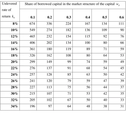
Now let us carry out an analysis of sensitivity of the approximate life of a project generating

positive cash flows depending on parameters k₀ and wd at typical (for the Russian

Federation) tax rate of 20%.

Table 1 - Analysis of sensitivity of the maximum time of an investment project, during which

the convergence of the algorithm is guaranteed, depending on parameters k0 and wd

Unlevered

rate of

return k0

Share of borrowed capital in the market structure of the capital wd

0.1 0.2 0.3 0.4 0.5 0.6

8% 674 336 224 167 134 111

10% 549 274 182 136 109 90

12% 465 232 154 115 92 76

14% 406 202 134 100 80 66

16% 361 180 119 89 71 59

18% 326 162 108 80 64 53

20% 299 149 99 74 59 49

22% 276 137 91 68 54 45

24% 257 128 85 63 50 42

26% 241 120 79 59 47 39

28% 227 113 75 56 44 37

30% 215 107 71 53 42 35

32% 205 102 67 50 40 33

34% 196 97 64 48 38 31

The table above provides a rough estimate of the limit life (years) of the forecasted

period for an investment project or a company generating positive cash flows, during which

the algorithm guarantees a uniqueness solution.

The unlevered rate k0 for companies generating cash flows exceeds 25% extremely

seldom; and the share of debt in the market structure of capital of such companies exceeds

50% on equivalently rare occasions.

This means that for a vast majority of actually existing companies generating only

positive cash flows the algorithm is characterized by convergence, since in most cases

forecasted periods for evaluation of companies generating cash flows do not exceed the

companies, for which cash flow duration does not exceed the maximum time of the project

(company).

However, for companies, which generate not only positive cash flows, this statement

is not true. Duration for such companies may exceed the maximum time (n) of the project

(company). In the work by (Limitovsky M.A., Minasyan V.B. 2010) we did not obtain the

sufficient condition for convergence of the iterative algorithm for companies generating not

only positive cash flows, because the authors failed to get estimates from a higher level (or

find another such valuation in literature) for the duration of a cash flow with other than

positive components of such cash flow. To overcome this difficulty, the following assertion

was proved in the work:

Assertion:

The following inequality is true for the duration of a cash flow which includes other

than positive components:

V V n n Dur   

 ( 1) ,

(23)

Where n = full time of existence of the cash flow; V = present (zero-moment) sum total of

values of modules of negative elements of the cash flow.

Proof

Let's assume that in k periods from n periods of existence of the cash flow, the cash

flows are negative, and in the rest (n – k) periods, they are positive. Periods with negative cash flows we will mark as i1,i2,...,ik ; whereas periods with positive cash flows, accordingly,

we will mark as ik1,ik2,...,in.

Then, the formula for determining duration will look as follows:





1 (1 )

1 ) 1 ( | | 1 .

Now we will introduce the designations:

j j j i i i WACC FCF V w ) 1 ( | | 1   

j j j i i i WACC FCF V w ) 1 ( 1  

 _{for j = 1, 2,…, k.}

Then, it is clear that the following equalities are true:

... ... 1

2 1 2

1        

      



 k n

k

k i i i

i i

i w w w w w

w

(24)

Duri1wi1 i2wi2 ...ikwik ik1wik1 ik2wik2 ...inwin

(25)

From the equation (25), it obviously follows that:

... ( ... ) 2 1 2 1      _{      }   _{ } n k k

k i i i

i i

i w w n w w w

w

Dur .

Then, using simple conversions and (25) several times, we will get:

                

 k n

k

k i i i

i i

i w w w w w

w

Dur ... ...

2 1 2

1     

     ... ) )( 1 ( 2

1 k n

k i i

i w w

w n

=1( 1)( _  _ ... )

2

1 k n

k i i

i w w

w n

1    ...  ( 1)( _  _ ... )

2 1 2

1 i ik ik ik in

i w w n w w w

w     

k

i i

i w w

w ... 2 1 = _{  }  _  _{ }  _   ... ) )( 2 ( 2 2

1 k n

k i i

i w w

w

n     

k

i i

i w w

w ... 2 1 = _{ } _  _{ }  _{ }  _  _{ }  _   ... ) )( 2 ( ... 2 2 1 2

1 i ik ik ik in

i w w n w w w

w 2(    ... )

2

1 i ik

i w w

w

3( 3)( _  _ ... )

2

1 k n

k i i

i w w

w

n 2(   ... )

2

1 i ik

i w w

w ….=

n ( 1)( ... ).

2 1    _{  }   k i i

i w w

w n

Recalling the expressions for wi_j, we will get:

( 1) .

) 1 ( | | 1 ) 1 ( 1 V V n n WACC FCF V n n Dur k j i i j j         



The assertion is thus proven.

If we use (22) and the proven assertion, it will be clear that trueness of inequality (22) for

such companies will be guaranteed if the following inequality is true:

. ) 1 ( 1 0  V V n n WACC k Durper     

) ) 1 ( ( 1 1 0 V V WACC k Dur V V n per     

  (26)

Inequality (26) constitutes a sufficient condition for convergence of our recurrent process. If

we substitute expressions for Durper and WACC into this inequality, this sufficient condition

for convergence (and, accordingly, for existence and uniqueness of the optimum

purpose-oriented capital structure) may be re-formulated as follows:

( 1 (1 ) ).

1 1 0 0 V V T w k T w k V V n d d         (27)

Now let us check the realizability of the sufficient condition for convergence of our iterative

process for companies which will, in future, generate not only positive cash flows.

Let us consider the following values: T=0.20, k0 0.25 , wd 0.5. Also, let us assume that

5 . 0   V V .

Let us mark, asV, the sum of values of positive components of the cash flow as

of the present moment (moment zero). The latter equality is equivalent to_  _  0.5

 V V V , or   V 3 1

V- , which looks rather realistic.

By substituting the selected parameter values into inequality (27), we will obtain:

). 5 . 0 20 . 0 5 . 0 25 . 0 ) 20 . 0 5 . 0 1 ( 25 . 0 1 ( 5 . 0 1 1 _         n

or n0.666(490.5)where  = any figure less than 1 but arbitrarily close to it. This

means that if the forecast period n for the project under the specified conditions is equal to

approximately 33 years or less, then the condition (27) will be met, and the algorithm will

provide a single and unique solution.

Now let us investigate the behavior of the right-hand portion of inequality (27) at all possible

realistic values of parameters k0 , wd and V

V

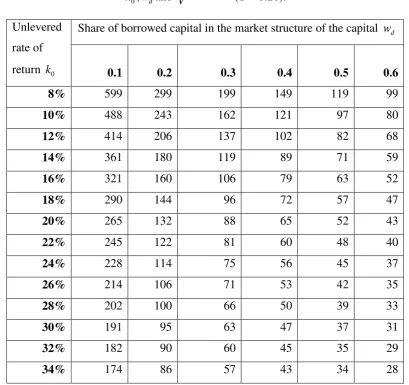
Table 2 - Analysis of sensitivity of the maximum time of an investment project, during which

the convergence of the algorithm is guaranteed, depending on parameters

0

k ,wdand

125 . 0





V V

(T = 0.20).

Unlevered

rate of

return k0

Share of borrowed capital in the market structure of the capital wd

0.1 0.2 0.3 0.4 0.5 0.6

8% 599 299 199 149 119 99

10% 488 243 162 121 97 80

12% 414 206 137 102 82 68

14% 361 180 119 89 71 59

16% 321 160 106 79 63 52

18% 290 144 96 72 57 47

20% 265 132 88 65 52 43

22% 245 122 81 60 48 40

24% 228 114 75 56 45 37

26% 214 106 71 53 42 35

28% 202 100 66 50 39 33

30% 191 95 63 47 37 31

32% 182 90 60 45 35 29

34% 174 86 57 43 34 28

Table 3 - Analysis of sensitivity of the maximum time of an investment project, during which the convergence of the algorithm is guaranteed, depending on parameters

0

k ,wdand

25 , 0





V V

(T = 0.20).

Unlevered

rate of

return k0

Share of borrowed capital in the market structure of the capital wd

0.1 0.2 0.3 0.4 0.5 0.6

10% 439 219 146 109 87 72

12% 372 186 123 92 74 61

14% 325 162 107 80 64 53

16% 289 144 96 71 57 47

18% 261 130 86 64 51 43

20% 239 119 79 59 47 39

22% 221 110 73 54 43 36

24% 206 102 68 51 40 33

26% 193 96 64 47 38 31

28% 182 90 60 45 35 29

30% 172 86 57 42 34 28

32% 164 81 54 40 32 26

34% 157 78 51 38 30 25

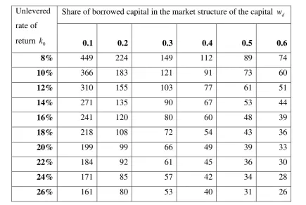
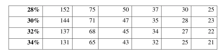
Table 4 - Analysis of sensitivity of the maximum time of an investment project, during which the convergence of the algorithm is guaranteed, depending on parameters

0

k ,wdand

5 . 0





V V

(T = 0.20).

Unlevered

rate of

return k0

Share of borrowed capital in the market structure of the capital wd

0.1 0.2 0.3 0.4 0.5 0.6

8% 449 224 149 112 89 74

10% 366 183 121 91 73 60

12% 310 155 103 77 61 51

14% 271 135 90 67 53 44

16% 241 120 80 60 48 39

18% 218 108 72 54 43 36

20% 199 99 66 49 39 33

22% 184 92 61 45 36 30

24% 171 85 57 42 34 28

28% 152 75 50 37 30 25

30% 144 71 47 35 28 23

32% 137 68 45 34 27 22

34% 131 65 43 32 25 21

Table 5 - Analysis of sensitivity of the maximum time of an investment project, during which the convergence of the algorithm is guaranteed, depending on parameters

0

k ,wdand

1





V V

(T = 0.20).

Unlevered

rate of

return k0

Share of borrowed capital in the market structure of the capital wd

0.1 0.2 0.3 0.4 0.5 0.6

8% 337 168 112 84 67 56

10% 275 137 91 68 55 45

12% 233 116 77 58 46 38

14% 203 101 67 50 40 33

16% 181 90 60 45 36 30

18% 163 81 54 40 32 27

20% 150 75 50 37 30 25

22% 138 69 46 34 27 23

24% 129 64 43 32 25 21

26% 121 60 40 30 24 20

28% 114 57 38 28 22 19

30% 108 54 36 27 21 18

32% 103 51 34 25 20 17

34% 98 49 32 24 19 16

Table 6 - Analysis of sensitivity of the maximum time of an investment project, during which the convergence of the algorithm is guaranteed, depending on parameters

0

k ,wdand

2





V V

Unlevered

rate of

return k0

Share of borrowed capital in the market structure of the capital wd

0.1 0.2 0.3 0.4 0.5 0.6

8% 225 112 75 56 45 37

10% 183 92 61 46 37 30

12% 155 78 52 39 31 26

14% 136 68 45 34 27 22

16% 121 60 40 30 24 20

18% 109 54 36 27 22 18

20% 100 50 33 25 20 17

22% 92 46 31 23 18 15

24% 86 43 29 21 17 14

26% 81 40 27 20 16 13

28% 76 38 25 19 15 13

30% 72 36 24 18 14 12

32% 69 34 23 17 14 11

34% 66 33 22 16 13 11

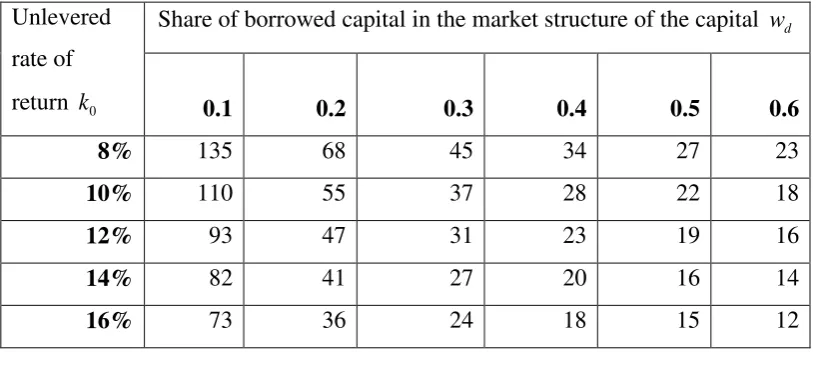
Table 7 - Analysis of sensitivity of the maximum time of an investment project, during which

the convergence of the algorithm is guaranteed, depending on parameters в

0

k ,wdand

4





V V

(T = 0.20).

Unlevered

rate of

return k0

Share of borrowed capital in the market structure of the capital wd

0.1 0.2 0.3 0.4 0.5 0.6

8% 135 68 45 34 27 23

10% 110 55 37 28 22 18

12% 93 47 31 23 19 16

14% 82 41 27 20 16 14

18% 66 33 22 16 13 11

20% 60 30 20 15 12 10

22% 56 28 19 14 11 9

24% 52 26 17 13 10 9

26% 49 24 16 12 10 8

28% 46 23 15 12 9 8

30% 43 22 15 11 9 7

32% 41 21 14 10 8 7

34% 40 20 13 10 8 7

The unlevered rate k0 for companies generating exceeds 25% extremely seldom; and

the share of debt in the market structure of capital of such companies exceeds 50% on

equivalently rare occasions.

The valuation practice shows that the share of the discounted absolute value of the

negative portion of cash flows of such companies in their total discounted cash flows _V

V

seldom goes beyond the limits of 0.125 thru 4. We can see that for projects (businesses) with

forecasted periods of 599 thru 7 years, convergence of the iterative process to the single

solution is guaranteed. Projects with the minimum guaranteed forecasted period of

convergence correspond to the maximum (from those considered) unlevered rate k0= 34%,

the maximum (from those considered) debt share of 0.6, and the maximum (of those

considered) discounted value of negative cash flow in their total discounted cash flows

4





V V

. Such combination has extremely low probability; but even in such a case,

convergence of the iteration process is guaranteed for forecasted periods of up to 7 years.

This means that for a vast majority of really existing companies, convergence of the

iteration algorithm is guaranteed by this criterion.

Convergence may be basically proven for other types of projects/companies (e.g. for a

company, which is an actual option or an economically separate project, etc). And though this

has not been done at this stage of the investigation, our multifarious applications of the

suggested algorithms in real projects testify to the fact that they almost always provide the

Conclusion

The difficulties in calculation of the capital structure, financial leverage, and weighted

average capital cost consist in the fact that to evaluate a project or a company one should

know the market structure of its capital; whereas, to obtain a reasonable market structure of

the capital, valuation results shall be available ((NPV or value of the company). To settle this

problem, in article suggest using iterative algorithms for calculating the structure and

weighted average capital cost for a company generating cash flows. These algorithms are

easily implementable using the popular EXCEL software. The article specifies advantages of

such algorithms in comparison with the famous Evans-Bishop and Pratt-Martin iterative

techniques. It is proven the suggested algorithms, in the vast majority of real situations, have a

single and unique solution for valuation calculations.

The general character of the proven criterion should be noted. In this work, the final

numerical test of convergence of the iterative process to a single solution is proven based on

notions of the reasonable area of measuring the key parameters which affect the convergence

of iterations in the Russian practice (e.g. the chosen tax rate is T = 0.20 etc.). However, using

this criterion and notions of the reasonable area of measuring the respective parameters in any

other countries, one can also verify, for which companies this algorithm will guarantee

convergence to the single solution determining the reasonable structure of capital of each

specific company.

References:

Damodaran A. (2004), Investment evaluation: Tools and methods for valuation of any assets,

Alpina Business Books, Moscow, Russia.

F.Ch. Evans, D.M. Bishop (2004), Valuation of companies during mergers and acquisitions.

Creation of cost in private companies, Alpina Publisher, Moscow, Russia.

Guidelines for evaluation of efficiency of investment projects. (2000), Economics, Moscow,

Russia.

Hamada R. (1972), «The effect of the firm’s capital structure on the systematic risk of

Holden C.W. (2004), Spreadsheet modeling in corporate finance, Prentice Hall, New Jercey.

Kolmogorov A.N., Fomin S.V. (1972), Elements of theory of functions and functional

analysis, Nauka, Moscow, Russia.

Limitovsky M.A. (2004), Investment projects and real options at emerging markets, Delo,

Moscow, Russia.

Limitovsky M.A., Minasyan V.B. (2010), «Development and implementation of iteration

algorithms for determining capital structure and valuation of capital cost», Management accounting and finance, 3, pp. 162-183.

Lumby S., Jones C. (2004), Corporate finance. Theory & practice, Thomson learning,

London.

Pratt Sh. (2006), Cost of capital, Quinto Consulting, Moscow, Russia.

Lumby S., Jones C. (2004), Corporate finance. Theory & practice, Thomson learning,

London.

Peterson D. and Peterson P. (1996), Company Performance and Measures of Value Added,

The Research Foundation of the Institute of Chartered Financial Analysts,