Dynamic Analysis of the Turnout Diverging Track for HSR with Variable Curvature Sections

ISSN Online: 2331-4249 ISSN Print: 2331-4222

Dynamic Analysis of the Turnout Diverging

Track for HSR with Variable Curvature Sections

Wladyslaw Koc, Katarzyna Palikowska

Department of Rail Transport and Bridges, Gdansk University of Technology, Gdansk, Poland

Abstract

The paper presents an analytical method of identifying the curvature of the turnout diverging track consisting of sections of varying curvature. Both li-near and nonlili-near (polynomial) curvatures of the turnout diverging track are identified and evaluated in the paper. The presented method is a universal one; it enables to assume curvature values at the beginning and end point of the geometrical layout of the turnout. The results of dynamics analysis show that widely used in railway practice, clothoid sections with nonzero curvatures at the beginning and end points of the turnout lead to increased dynamic in-teractions in the track-vehicle system. The turnout with nonlinear curvature reaching zero values at the extreme points of the geometrical layout is indi-cated in the paper as the most favourable, taking into account dynamic inte-ractions occurring in the track-vehicle system.

Keywords

Railway Turnouts, Curvature Modelling, Dynamics Analysis

1. Introduction

Typical, used since the beginning of railway engineering, geometrical layout of the turnout diverging track consists of a single circular arc without transition curves. It introduces sudden, abrupt changes of the horizontal curvature of the layout at the beginning and end of the turnout diverging track, which increases dynamic interactions in the track-vehicle system, particularly unfavourable in high speed rail (HSR). Investigation and evaluation of geometrical layouts of the turnout diverging track are still a current issue.

Recently, aiming at smoothing changes of the curvature at the neuralgic re-gions of the turnout diverging track, the clothoid sections have been introduced at both sides of the circular arc [1] [2] [3]. The curvature of the applied clothoid How to cite this paper: Koc, W. and

Palikowska, K. (2017) Dynamic Analysis of the Turnout Diverging Track for HSR with Variable Curvature Sections. World Journal of Engineering and Technology, 5, 42-57.

https://doi.org/10.4236/wjet.2017.51005

Received: December 9, 2016 Accepted: February 18, 2017 Published: February 21, 2017

Copyright © 2017 by authors and Scientific Research Publishing Inc. This work is licensed under the Creative Commons Attribution International License (CC BY 4.0).

http://creativecommons.org/licenses/by/4.0/

sections in many cases does not reach zero value at the extreme points (i.e. at the beginning and end points of the turnout). The paper presents the evaluation of the selected geometrical layouts of the turnout diverging track to indicate the most favourable solution for HSR.

In the turnout with linear curvature sections, a diverging track is divided into three zones (Figure 1):

• _{a beginning zone of the length} l₁, in which curvature increases linearly from

1 1 1

k R

= _(or k₁=0) to 2 2 1

k R

= _,

• _{a middle zone of the length} l₂ with constant curvature 2 2 1

k R

= _,

• _{an end zone of the length} l₃, in which curvature decreases linearly from

2 2 1

k R

= _{, to} 3 3 1

k R

= _(or k₃=0).

The various values of curvature and length of each section can be applied in the designing process. Curvature of the turnout diverging track is described by an analytical function k l

( )

, where l stands for the length of the curve.

This paper presents the identification of analytical functions k l

( )

for linear curvature sections (i.e. clothoid sections) as well as for nonlinear curvature sec-tions in the polynomial form. The identified curvatures have been compared using the dynamic model, described in [4], to find out the most favorable solu-tion from the point of view of minimizing the dynamic effects.

In this paper, the Cartesian coordinates of the turnout diverging tracks are not presented. The method of the identification of the Cartesian coordinates from the curvature k l

( )

is described in [4]. The determination of parametric equa-tions x l

( )

and y l

( )

requires the expansion of the integrands into Taylor se-ries [5] using Maxima package [6].

2. Application of the Linear Curvature Sections

2.1. Solution for the Beginning Zone

[image:2.595.226.520.556.700.2]

In the beginning zone of the turnout the considered issue is identified by boundary

conditions [2]

( )

( )

1 12

0

k k

k l k

 =



 ₌

 (1) and a differential equation

( )

0

k′′ l = . (2)

After determining the constants, the solution of the differential problem (1), (2) is as follows:

( )

2 1

1 1

k k

k l k l

l

−

= + . (3)

The slope of the tangent at the end of the zone, for l=l1, is defined by the formula:

( )

1 2

1 1

2

k k

l l

θ = + . (4)

2.2. Solution for the Middle Zone

In the circular arc zone, i.e. for l∈ l l1,1+l2 , curvature is constant:

( )

2

k l =k . (5)

At the end of circular arc the slope of the tangent is defined by the formula:

(

)

1 2

1 2 1 2 2

2

k k

l l l k l

θ + = + + ⋅ . (6)

2.3. Solution for the End Zone

In the end zone of the turnout the following boundary conditions are adopted:

(

)

(

11 22 3

)

2 3

k l l k k l l l k

 + =



 _{+ + =}

 (7)

for the differential Equation (2). After determining the constants, the solution of the differential problem (2), (7) is as follows:

( )

3 2

(

)

3 2

2 1 2

3 3

k k k k

k l k l l l

l l

− −

= − + + _{. (8)}

The slope of the tangent at the end of the turnout is defined by the formula:

(

)

1 2 2 3

1 2 3 1 2 2 3

2 2

k k

k k

l l l l k l l

θ + + = + + + + _{, (9)}

from which the turnout angle 1

n can be obtained as

(

1 2 3

)

1 tan

n

l l l

θ =

+ + . (10)

3. Application of the Nonlinear Curvature Sections

sides of the circular arc and the assumption of zero curvature value at the ex-treme points (i.e. the turnout beginning and end points) of the geometric layout are worth considering.

3.1. Solution for the Beginning Zone

The following boundary conditions have been adopted:

( )

( )

( )

( )

1 1 2

2 1

1 1

0

0 0

k k k l k

k k

k C k l

l

 = =



−

 ′ = ′ =

 

(11)

to the differential equation

( )4

_{( )}

0

k l = (12)

with assumption, that coefficient C≥0.

As a result of solving the differential problem (11), (12) the following curva-ture has been obtained:

( )

(

)

(

)

2

(

)

3

1 2 1 2 2 1 3 2 1

1 1 1

2 3 2

C C C

k l k k k l k k l k k l

l l l

− −

= + − − − + − . (13)

Function k l

( )

describing the curvature in the considered zone should be monotonic and should increase for l>0. In order to obtain a feasible solution the coefficient C should be properly adjusted. It has been shown, that the appro-priate C∈ 1.5; 3 . Taking into account the length of the parametric curve (13) and a curve of linear curvature (i.e. generalized clothoid) the most favourable assumption seems to be C = 1.5. Curvature k l

( )

in this case is as follows:

( )

(

)

(

)

3

1 2 1 3 2 1

1 1

3 1

2 2

k l k k k l k k l

l l

= + − − − _{. (14)}

At the end of the zone, for l=l1, the slope of the tangent is described by the formula:

( )

1 2

1 1

3 5

8

k k

l l

θ = + _{. (15)}

3.2. Solution for the Middle Zone

Similarly to the middle zone described in the section 2.2, i.e. for l∈ l l1,1+l2 ,

the curvature is constant k l

( )

=k2. The slope of the tangent at the end of the

circular arc, for l= +l1 l2, is described by the formula:

(

)

1 2

1 2 1 2 2

3 5

8

k k

l l l k l

θ + = + + ⋅ . (16)

3.3. Solution for the End Zone

Assuming the boundary conditions:

(

)

(

)

(

)

(

)

1 2 2 1 2 3 3

3 2

1 2 1 2 3

3

0

k l l k k l l l k

k k

k l l k l l l C

l

 + = + + =



−

 ′ + = ′ + + =

 

for the differential Equation (12) the following solution has been obtained:

( )

2 3

1 2 3 4

k l = +c c l+c l +c l (18)

where

(

)

2

(

) (

3

)

1 2 2 1 2 3 1 2 3 2

3 3

3 C 2 C

c k l l l l k k

l l

 − − 

= +_ + + + _ −

 

(

_{) ( ) ( )( ) (}

2

₎

2 2 1 2 3 1 2 3 2

3 3

2 3 C 3 2 C

c l l l l k k

l l − −   = −_ + + + _ −  

(

_{) ( ) (}

₎

3 2 3 1 2 3 2

3 3

3 2

3 C C

c l l k k

l l −  −  =_ + + _ −  

(

)

4 3 3 2

3 2

.

C

c k k

l

−

= − −

Assuming C = 1.5 the following coefficient formulas have been obtained:

(

)

2

(

) (

3

)

1 2 2 1 2 3 1 2 3 2

3 3

3 1

2 2

c k l l l l k k

l l

 

= +_ + + + _ −

 

(

)

(

) (

2

)

2 2 1 2 3 1 2 3 2

3 3

3 3

2

c l l l l k k

l l

 

= −_ + + + _ −

 

(

) (

)

3 2 3 1 2 3 2

3 3

3 3

2 2

c l l k k

l l

 

=_ + + _ −

 

(

)

4 3 3 2

3 1

. 2

c k k

l

= − −

The slope of the tangent at the end of the turnout, for l= + +l1 l2 l3, is de-fined by the formula:

(

)

1 2 3 2

1 2 3 1 2 2 3

3 5

3 5

8 8

k k

k k

l l l l k l l

θ + + = + + ⋅ + + _{. (19)}

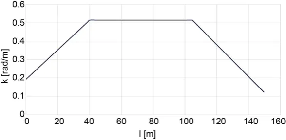
In Figure 2 the curvature of the turnout diverging track (for C = 1.5) with nonlinear curvature sections has been shown. The geometric parameters of the turnouts presented in Figure 1 and Figure 2 are conform.

4. Selection of the Geometrical Layouts of Turnout

Diverging Tracks

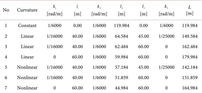
In order to ensure a reliable comparative analysis of the geometrical layouts pre-sented in Table 1, the following common assumptions have been adopted:

• _{the turnout angle 1:n , where n = 50,}

• _{the curvature values} k₁, k2 and k3 are common to all turnouts, • _{the circular arc radius} R₂=6000 m,

• _{the length of the beginning zone} l₁ and the end zone l3 are similar and ensures the fulfillment of the kinematic conditions,

[image:6.595.208.536.68.224.2]

Figure 2. Curvature of the turnout diverging track (nonlinear curvature sections for C = 1.5)

(

R1=16000 m, l1=40 m,R2=6000 m, l2=57.184 m, l3=45 m,R3=25000 m

)

.

Table 1. Geometric parameters of the selected turnouts (the turnout angle 1:50).

No Curvature k1

[rad/m]

1

l

[m]

2

k

[rad/m]

2

l

[m]

3

l

[m]

3

k

[rad/m] L [m]

1 Constant 1/6000 0.00 1/6000 119.984 0.00 1/6000 119.984 2 Linear 1/16000 40.00 1/6000 64.584 45.00 1/25000 149.584 3 Linear 1/16000 40.00 1/6000 62.484 60.00 0 162.484 4 Linear 0 60.00 1/6000 59.984 60.00 0 179.984 5 Nonlinear 1/16000 40.00 1/6000 57.184 45.00 1/25000 142.184 6 Nonlinear 1/16000 40.00 1/6000 51.859 60.00 0 151.859 7 Nonlinear 0 60.00 1/6000 44.984 60.00 0 164.984

The highest velocity on a circular arc without superelevation (i.e. in the mid-dle zone) results from the following condition:

2

per 1 3, 6

m

V

a a

R

 

=_{ } ≤

  ,

while in the extreme zones the condition is as follows

( )

per

d

max max

3, 6 d V

a l l

ψ = ≤ψ

where:

V—train velocity [km/h], R—circular arc radius [m],

m

a —acceleration on circular arc [m/s2],

per

a —permissible value of acceleration on circular arc [m/s2],

( )

a l —function describing lateral acceleration in the zones of changing cur-vature,

ψ _{—rate of acceleration changes in the zone of changing curvature [m/s}3_].

per

ψ

_{—permissible value of parameter} ψ [m/s3_].

It is assumed that 2

per 0.6 m s

a = and 3

per 0.5 m s

[image:6.595.208.539.294.447.2]

On a circular arc without transition curves (turnout 1) the acceleration changes linearly from 0 to am along the length of the rigid base of wagon lb. Taking

into account

( )

2 1

3, 6 b

V

a l l

Rl

 

= _ _ for l∈ 0,l_b

with condition

3

per 1 3, 6 b

V Rl

ψ

=_ _ ≤

ψ

 

the limit of the velocity Vmax is obtained as follows

3

max 3, 6 b per

V = ⋅ R l⋅ ⋅ψ . (20)

On a circular arc in the middle zone with sections of changing curvature in the beginning and end zones the limit of the velocity is described by the formula

max 3, 6 2 per

V = R ⋅a (21)

In the beginning zone where curvature changes linearly a rate of acceleration changes ψ is constant. In this zone the following condition should be fulfilled:

3

per

2 1 1

1 1 1

3, 6 V

R R l

ψ =_ _ _ − _ ≤ψ

    ,

from which the minimal length l1 of the beginning zone can be determined:

3

1

2 1 per

1 1 1

3, 6 V l

R R ψ

 

 

≥_{  } − _

    . (22)

Nonlinear curvature (polynomial) induces changing rate of acceleration changes ψ _{along the length of the turnout. The following condition should be} fulfilled:

3

2

max 3 per

2 1 1 1

1 1 3 3

max 1.5 .

3, 6 2 2

V

l

R R l l

ψ =    −  − ≤ ⋅ψ

 

   

 

An increase by 50% of the limit value

ψ

per is justified by the fact, that the value ψmaxoccurs only once (for l = 0), and next decreases, reaches at the end of the section (for l=l1) zero value. The condition (22) can be applied also for the end zone of the turnout.

For the assumed turnout angle 1:50 (i.e. n = 50) the following slope of the tangent has been obtained, using Equation (10):

(

1 2 3

)

1

arctan 0.019997 rad.

l l l

n

θ + + = =

Assuming lb =20 m for the turnout diverging track 1 (Table 1), using Equ-ation (20) the maximal velocity ,

max 140.9352 km h

R b

V = . The length of the

cir-cular arc is obtained as follows: l2= ⋅R θ

(

l1+ +l2 l3

)

=119.984 m. The velocity

limit in turnouts 2 ÷ 7 results from the Equation (21): Vmax =216 km h (in the comparative analysis of the turnouts, presented in section 6, it was assumed

200 km h

The geometrical parameters of the selected seven turnouts are presented in Table 1. The lengths of the sections l1 and l3 result from condition (22), while the length l2 results from the assumed slope of the tangent in the Equation (9) for linear curvature:

(

)

1 2 2 3

2 1 2 3 1 3

2 1

2 2

k k k k

l l l l l l

k θ

+ +

 

= _ + + − − _

  (23)

and in the Equation (19) for nonlinear curvature:

(

)

1 2 3 2

2 1 2 3 1 3

2 3 5 3 5 1 8 8 k k k k

l l l l l l

k θ

+ +

 

= _ + + − − _

 . (24)

The function of lateral acceleration a l

( )

along the layout, as proved in [4], results directly from the layout curvature k l

( )

. The assumed functions of lateral acceleration a l

( )

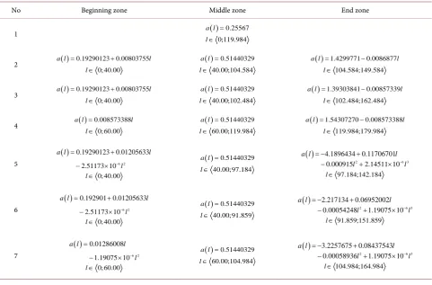
for selected turnouts are presented in Table 2.

5. The Dynamic Model

[image:8.595.203.538.136.216.2]

With increased speed requirements on railways, the dynamic effects minimiza-tion is a current issue, especially in HSR. Basing on the assumpminimiza-tion that hori-zontal curvature changes are a forcing factor of the lateral oscillations, selected seven geometrical layouts of the turnout diverging track are compared in terms on their impact on the dynamic interactions occurring in a rail-vehicle system. In the presented comparative analysis of the layouts, structural aspects of the rail

Table 2. Lateral acceleration a l

( )

[m/s2] along the three zones (length [m]) of the selected turnouts.

No Beginning zone Middle zone End zone

1 a l( )=0.25567

0;119.984 l∈

2 a l( )=0.19290123+0.00803755l

0; 40.00 l∈

( ) 0.51440329

a l =

40.00;104.584 l∈

( ) 1.4299771 0.0086877

a l = − l

104.584;149.584 l∈

3 a l( )=0.19290123+0.00803755l

0; 40.00 l∈

( ) 0.51440329

a l =

40.00;102.484 l∈

( ) 1.39303841 0.00857339

a l = − l

102.484;162.484 l∈

4 a l( )=0.008573388l

0; 60.00 l∈

( ) 0.51440329

a l =

60.00;119.984 l∈

( ) 1.54307270 0.008573388

a l = − l

119.984;179.984 l∈ 5 ( ) 6 2 0.19290123 0.01205633 2.51173 10

a l l

l − = + − × 0; 40.00 l∈

( ) 0.51440329

a l =

40.00;97.184 l∈

( )

2 6 3

4.1896434 0.11706701 0.000915 2.14511 10

a l l

l −l

= − + − + × 97.184;142.184 l∈ 6 ( ) 6 2 0.192901 0.01205633 2.51173 10

a l l

l − = + − × 0; 40.00 l∈

( ) 0.51440329

a l =

40.00;91.859 l∈

( )

2 6 3

2.217134 0.06952002 0.00054248 1.19075 10

a l l

l −l

= − + − + × 91.859;151.859 l∈ 7 ( ) 6 2 0.01286008 1.19075 10

a l l

l − = − × 0; 60.00 l∈

( ) 0.51440329

a l =

60.00;104.984 l∈

( )

2 63

3.2257675 0.08437543 0.00058936 1.19075 10

a l l

l −l

= − +

− + ×

[image:8.595.57.539.424.741.2]

vehicle are omitted.

A dynamic model with one degree of freedom, consisting of a mass with a spring and a damper is applied to compare the dynamic interactions occurring on the various turnout diverging tracks. An additional parameter—a length of the rigid base of a wagon has been introduced, which results in referring to the lateral acceleration of the wagon mass center (arithmetic mean of accelerations occurring in the front and rear bogies).

The lateral acceleration a t

( )

occurring along the turnout diverging track can be described by the separate functions dedicate for different turnout zones. As-suming constant velocity along the turnout, as it is done in this paper, function

( )

a l for each turnout zone is presented in Table 2. Considered case includes driven horizontal harmonic oscillations X [7] described by the equation

( )

( )

₍

₎

_{( )}

_{( )}

2

2 2

2

d d

2 d d

X t X t

u u X t a t

t

t + +

ω

+ = (25)

where:

D—Lehr’s damping coefficient,

ω

—free oscillation frequency,

2 1

D u

D

ω

=

− .

Lehr’s damping coefficient D is used as a damping measure in the railway en-gineering. In the presented paper D = 0.175 and ω = 3.5 π/s are assumed. The assumed value of D has been obtained in the experimental research presented in [8]. As proved in [9] this assumption has no impact on conclusions from the comparative analysis of dynamic properties of railway geometrical layouts.

The function of oscillations X t

( )

, describing lateral displacement of the ve-hicle under the force P t

( )

= ⋅m a t

( )

, is the solution to the differential Equation (25). The function X t

( )

is the resultant of the static component and the sys-tem oscillations. From the point of view of dynamic effects evaluation the resul-tant acceleration of oscillation motion av= X′′

( )

t is essential. The maximum amplitude of the acceleration of oscillating motion maxX′′ and indicator w_a

defined as follows

( )

0

0

d

k

l l

a l

w X t l

+

′′

=

_∫

₍₂₆₎

where:

0

l —the point at which curvature of the turnout diverging track changes,

k

l —the length of the section on which oscillations are damped,

are assumed as criteria of the dynamic effects evaluation presented in Section 6.

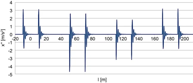
6. Results of the Dynamics Analysis

Figure 3. Lateral acceleration forcing the lateral oscillations for turnout 1.

Figure 4. Lateral acceleration forcing the lateral oscillations for turnout 2.

1).

The acceleration of oscillating motion X′′

( )

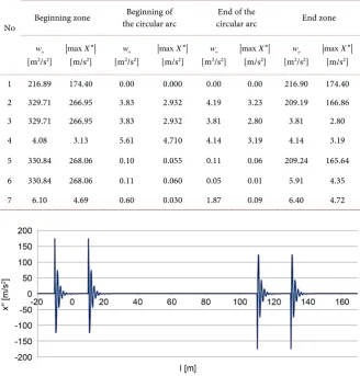
l , computed numerically using the dynamic model described in section 5, for the selected seven geometrical layouts of turnout diverging track (Table 2 and Table 3) is presented in Figures 5-12.

Apart from the beginning and end zones of the turnout diverging track, the dynamic interactions occur also at the beginning and end of the middle zone, as shown in Figure 7.

The comparative analysis of the selected layouts of the turnouts diverging track has been carried out using dynamic indicators: wa (26) and maxX′′,

based on acceleration of oscillating motion X′′

( )

l from Figures 5-12. The computed values of wa and maxX′′ for the selected seven turnouts are

pre-sented in Table 3.

[image:11.595.209.538.125.469.2]

Table 3. Dynamic indicators wa and amplitude of the acceleration of oscillating motion

( )

X′′ l for selected turnouts.

No

Zones of dynamic effects along the turnout diverging track

Beginning zone _{the circular arc} Beginning of _{circular arc} End of the End zone

a

w

[m2_/s2_]

maxX′′

[m/s2_] a

w

[m2_/s2_]

maxX′′

[m/s2_] a

w

[m2_/s2_]

maxX′′

[m/s2_] a

w

[m2_/s2_]

maxX′′

[m/s2_]

[image:11.595.208.539.125.466.2]

1 216.89 174.40 0.00 0.000 0.00 0.00 216.90 174.40 2 329.71 266.95 3.83 2.932 4.19 3.23 209.19 166.86 3 329.71 266.95 3.83 2.932 3.81 2.80 3.81 2.80 4 4.08 3.13 5.61 4.710 4.14 3.19 4.14 3.19 5 330.84 268.06 0.10 0.055 0.11 0.06 209.24 165.64 6 330.84 268.06 0.11 0.060 0.05 0.01 5.91 4.35 7 6.10 4.69 0.60 0.030 1.87 0.09 6.40 4.72

Figure 5. Acceleration of oscillating motion X′′

( )

l for turnout 1 (V = 141 km/h).

Figure 6. Acceleration of oscillating motion X′′

( )

l for turnout 2 (V = 200 km/h).

[image:11.595.215.539.504.642.2]

[image:12.595.211.537.71.216.2] [image:12.595.209.543.264.404.2]

Figure 7. Acceleration of oscillating motion X′′

( )

l in the middle zone of the turnout 2 (V = 200 km/h).

Figure 8. Acceleration of oscillating motion X′′

( )

l for turnout 3 (V = 200 km/h).

Figure 9. Acceleration of oscillating motion X′′

( )

l for turnout 4 (V = 200 km/h).

along the whole turnout diverging track; it is concerned layouts with sections of linear curvature (turnout 4—Figure 9) as well as layouts with sections of nonli-near curvature (turnout 7—Figure 12).

[image:12.595.211.536.438.578.2]

[image:13.595.210.538.70.199.2] [image:13.595.210.538.236.372.2]

Figure 10. Acceleration of oscillating motion X′′

( )

l for turnout 5 (V = 200 km/h).

[image:13.595.214.536.408.535.2]

Figure 11. Acceleration of oscillating motion X′′

( )

l for turnout 6 (V = 200 km/h).

Figure 12. Acceleration of oscillating motion X′′

( )

l for turnout 7 (V = 200 km/h).

slightly increase (Table 1).

The acceleration in oscillating motion X′′

( )

l occurring at the beginning and at the end of the middle zone is not dependent on the curvatures values k1 and

3

k , adopted in the beginning and the end zone of the turnout, but depends on

the curvature characteristics. Linear curvatures k1 and k3 (turnouts 2 ÷ 4, Figures 6-9) induce greater values of dynamic indicators (Table 3) than nonli-near ones (turnouts 5 ÷ 7, Figures 10-12).

and end zones (Table 3).

7. The Most Favourable Geometrical Layout of the

Turnout Diverging Track

As a result of dynamics analysis it has been proved that the most favourable dy-namic properties can be achieved by applying a nonlinear curvature in the be-ginning and end zones of the turnout diverging track and assuming zero curva-ture value at the extreme points of the geometrical layout.

Assuming k1=0 and k3 =0 the curvature k l

( )

of the turnout is defined as follows:

• _{in the beginning zone, for} l∈ 0,l₁ , based on the Equation (14) the follow-ing formula is obtained

( )

2 2 3

3

1 1

3

2 2

k k

k l l l

l l

= − ₍₂₇₎

• _{in the middle zone, i.e. for} l∈ l l₁,₁+l₂ , the curvature is constant

( )

2

k l =k

• _{in the end zone, for} l∈ l₁+l l₂,₁+ +l₂ l₃ the curvature is described by the Equation (18) with the following coefficient values:

(

)

2

(

)

3

1 2 2 1 2 3 1 2

3 3

3 1

1

2 2

c k l l l l

l l

  

 

= _ −_ + + + _

  

 

(

)

(

)

2

2 2 2 1 2 3 1 2

3 3

3 3

2

c k l l l l

l l

 

= _ + + + _

 

(

)

3 2 2 3 1 2

3 3

3 3

2 2

c k l l

l l

 

= − _ + + _

 

2

4 3

3 . 2

k c

l

=

The slope of the tangent at the end of the turnout, for l= + +l1 l2 l3, is as fol-lows

(

)

2

(

)

1 2 3 2 2 1 3

5 8

k

l l l k l l l

θ + + = + + . (28)

In Figure 13 the curvature of the most favorable turnout diverging track 7 is presented.

8. Conclusions

Typical turnout diverging track consists of a single circular arc without transi-tion curves. It introduces sudden, abrupt changes of the horizontal curvature of the layout at the beginning and end of the turnout diverging track, which in-creases dynamic interactions in the track-vehicle system, particularly unfavoura-ble in HSR.

[image:15.595.208.532.74.214.2]

Figure 13. Curvature of the turnout diverging track 7 (nonlinear curvature sections).

(

k1=0, l1=60 m,k2=1 6000 rad m , l2=44.984 m, l3=60 m,k3=0

)

.

model. The presented method enables to assume the curvature values at the be-ginning and end point of the geometrical layout of the turnout. The length of the circular arc is adjusted to obtain the assumed turnout angle.

Recently, aiming at smoothing changes of the curvature at the neuralgic re-gions of the turnout diverging track, the clothoid sections have been introduced at both sides of the circular arc. The curvature of the applied clothoid sections changes linearly but in many cases does not reach zero value at the extreme points (i.e. at the beginning and end points of the turnout). The results of dy-namics analysis presented in the paper show that clothoid sections with nonzero curvature at the beginning and end points of the turnout lead to increased dy-namic interactions in the track-vehicle system. Dydy-namic interactions can be de-creased by applying curvature reaching zero at the extreme points of the turnout.

The paper presents the evaluation of the selected seven geometrical layouts of the turnout diverging track and indicates the most favourable solution for HSR. The most favourable from the dynamic properties point of view is the turnout diverging track with nonlinear curvature reaching zero values at the extreme points of the turnout.

References

[1] Fei, W.Z. (2009) Major Technical Characteristics of High-Speed Turnout in France. Journal of Railway Engineering Society, 9, 18-35.

[2] Parsons Brinckerhoff for the California High-Speed Rail Authority (2009) Technical Memorandum: Alignment Design Standards for High-Speed Train Operation. [3] Wang, P. (2015) Design of High-Speed Railway Turnouts. Theory and Applications.

Elsevier Science & Technology, Oxford, United Kingdom.

[4] Koc, W. (2014) Analytical Method of Modelling the Geometric System of Commu-nication Route. Mathematical Problems in Engineering, 2014, Article ID: 679817.

https://doi.org/10.1155/2014/679817

[5] Korn, G.A. and Korn, T.M. (1968) Mathematical Handbook for Scientists and En-gineers. McGraw-Hill Book Company, New York, USA.

[6] Maxima Package. http://maxima.sourceforge.net

Ebook Download, Prentice Hall. http://bit.ly/enmechdynamics14thPDF

[8] Varga, J., et al. (1980) Analysis of Admissible Influence on Railway Vehicle Moving Along Transition Curves with Linear (Clothoid) and Cosine Curve Geometry and Along Turnouts with Great Radii (in Hungarian). The Sci. Works of Railway Insti-tute, Budapest.

[9] Koc, W. and Palikowska, K. (1999) Intelligent Modelling of the Railway Track Layouts Using Dynamic Criteria. International Conference of Modelling and Man-agement in Transportation, Poznan-Cracow, Poland, 15-16 October 1999, 245-250.

Submit or recommend next manuscript to SCIRP and we will provide best service for you:

Accepting pre-submission inquiries through Email, Facebook, LinkedIn, Twitter, etc. A wide selection of journals (inclusive of 9 subjects, more than 200 journals)

Providing 24-hour high-quality service User-friendly online submission system Fair and swift peer-review system

Efficient typesetting and proofreading procedure

Display of the result of downloads and visits, as well as the number of cited articles Maximum dissemination of your research work