Estimating the dose response function through the GLM approach

(1)

Munich Personal RePEc Archive

Estimating the dose-response function

through the GLM approach

Guardabascio, Barbara and Ventura, Marco

Italian National Institute of Statistics (ISTAT), Italian National

Institute of Statistics (ISTAT)

13 March 2013

(2)

Estimating the dose-response function

through the GLM approach

Barbara Guardabascio

ISTAT, Italian National Institute of Statistics Rome, Italy

[email protected] Marco Ventura

ISTAT, Italian National Institute of Statistics Rome, Italy

[email protected]

Abstract. This paper revises the estimation of the dose-response function

as in Hirano and Imbens (2004) by proposing a flexible way to estimate the generalized propensity score when the treatment variable is not necessarily normally distributed. We also provide a set of programs that accomplish this task by using the GLM in the first step of the computation.

Keywords: generalized propensity score, GLM, dose-response, continuous

treatment, bias removal

1 Introduction

How effective are policy programs with continuous treatment exposure? An-swering this question essentially amounts to estimate a dose-response function as proposed in Hirano and Imbens (2004). Whenever doses are not randomly assigned, but are given under experimental conditions, estimation of a dose-response function is possible using the Generalized Propensity Score (GPS). The GPS for continuous treatment is an extension of the popular propensity score methodology for binary treatments (Rosenbaum and Rubin, 1983, 1984) and multi-valued treatments (Imbens, 2000; Lechner, 2001). Indeed, Hirano and Imbens show that the GPS has a balancing property similar to the bi-nary propensity score. Conditional on observable characteristics, the level of the treatment can be considered as random for units belonging to the same GPS strata. It means that adjusting for the GPS removes all biases associ-ated with differences in the covariates. Since its formulation, the GPS has been repeatedly used in observational studies andad hoc programs have been pro-vided for STATA usersdoseresponse.adoandgpscore.ado by Bia and Mat-tei (2008), henceforth BM. However, many applied works (Fryges and Wagner, 2008; Fryges, 2009) remark that the treatment variable may be not normally distributed. In this case the BM programs are not usable as they do not allow for different distribution assumptions other than the normal density.

(3)

Models estimator, GLM, in the first step instead of the Maximum Likelihood, ML, for normal distribution.

In order to easily compare our programs with the BM ones, we use the same dataset used by BM and originally collected by Imbens et al (2001). The sample is made up of individuals winning the Megabucks lottery in Massachusetts in the mid-1980’s. The main source of potential bias is the unit and item nonresponse. Hirano and Imbens (2004) claim that it is possible to prove that the nonresponse was non-random. The missing data imply that the amount of the prize is po-tentially correlated with background characteristics and potential outcomes. It may be useful to remind that using these bias reducing techniques, it is possible to reduce, not to eliminate the bias generated by unobservable heterogeneity. The extent to which unconfoundedness holds, namely the extent to which the bias is reduced, depends on the quality of the database used to compute the GPS. This caveat is independent of the particular distribution function one is willing to assume for the treatment variable.

The reminder of the paper proceeds as follows. Section 2 briefly reviews the estimation of the dose-response function. Section 3 introduces the GLM and explains how to use it to fit the GPS. Section 3.1. analyzes flogit, a special case of particular interest in economics. Section 4 describes how the programs work step by step. Section 5 and 6 list the syntax and the options, respectively. Section 7 presents an application of the programs using some non-normal distribution of the treatment variable. Section 8 concludes.

2 A brief review of the econometrics of the

dose-response function

Let us define a set of potential outcomes{Yi(t)} fort∈ T, where T represents

the continuous set of potential treatments defined over the interval [t0, t1], and

Yi(t) is referred to as the unit-level dose-response function.

Let us suppose to have a random sample of N units. For each unit i we observe a k×1 vector of pre-treatment covariates, Xi, the level of the

treat-ment delivered,Ti, and the outcome corresponding to the level of the treatment

received, Yi =Yi(Ti). We are interested in the average dose-response function

ψ(t) =E[Yi(t)].

Under some regularity conditions1_of_{_Y

i(t)},Xi, andTiHirano and Imbens

define the propensity function as the conditional density of the actual treatment given the covariates. More in detail, if we define as r(t, x) = fT|X(t|x) the

conditional density function of the treatment given the covariates, then the GPS is

R=r(T|X)

The balancing property can be defined similarly to the binary case. That is, within strata with the same value ofr(t, x),the probability thatT =tdoes

1_{For each}_i_,_{_Y

i(t)},XiandTiare supposed to be defined on a common probability space, Ti is continuously distributed with respect to Lebsgue measure onT, andYi=Yi(Ti) is a

(4)

not depend on the value ofX:

X⊥1{T =t}|r(t, x)

This balancing property, along with unconfoundedness implies that assignment to treatment is unconfounded given the GPS. If weak unconfoundedness as-sumption holds, given the pre-treatment variablesX, we have:

Y(t)⊥T|X ∀t∈ T

then, for everyt

fT(t|r(t, X), Y(t)) =fT(t|r(t, X))

this means that the GPS can be used to eliminate any bias associated with differences in the covariates (for a formal proof see Theorem 2.1 and 3.1 of Hirano and Imbens, 2004). Therefore, the dose-response function can be obtained as

γ(t, r) = E[Y(t)|r(t, X) =r] =E[Y|T =t, R=r] (1)

ψ(t) = E[γ(t, r(t, X))] (2)

Practical implementation of the GPS is accomplished in three steps2_. In the first step the score r(t, x) is estimated. In the second step the con-ditional expectation of the outcome as a function of two scalar variables, the treatment levelT and the GPSR, is estimated,E[Y|T =t, R=r]. In the third step the dose-response function,ψ(t) =E[(t, r(t, X))], t ∈ T , is estimated by averaging the estimated conditional expectation, ˆγ(t, r(t, X)), over the GPS at each level of the treatment one is interested in.

As the second and the third step in our programs replicate BM’s program, we refer to it for more details about these steps. While, we will devote more attention in explaining how our programs implement the first step to compute the scorer(t, x).

3 Estimation of the score through the GLM

In many economic applications T cannot be supposed to be normally dis-tributed and assuming a normal distribution of the treatment given the co-variates,Ti|Xi∼N(β′Xi, σ2) whereβ isk×1 vector of parameters, has several

drawbacks. The problem is not new in the econometric literature, think about count, binomial, fractional and survival data, just to cite a few (see Wooldridge 2002 for a comprehensive review of this topic). Taking into account what be-fore, we aim to go beyond these problems presenting a possible solution to the estimation of the GPS in these cases. Our idea consists in replacing the linear regression3_{by the GLM developed by McCullagh and Nelder (1989) in the first} step to estimate the dose-response, and to retrieve the GPS from the exponential

2_{Hirano and Imbens and BM use the notation}_µ_{instead of}_ψ_and_β_{instead of}_γ_{. We have}

slightly changed notation in order to avoid confusion in the following Sections.

3_{Precisely, the programs by BM estimate the GPS assuming}_T_|_X_{or some transformations}

(5)

family distribution. By using the GLM the modelling differs from the ordinary regression in two important respects. First, the distribution ofT is chosen from the exponential family. Thus, the distribution may not be normal or close to the normal and may be explicitly non-normal. Second, a transformation of the mean of the treatment is linearly related to the explanatory variables. These two basic ingredients of the GLM can be formalized as follows:

f(T) = c(T, φ)exp

_{T θ}₋_a₍_θ₎

φ

(3)

g{E(T)} = β′_X ₍₄₎

Equation (3) specifies that the distribution of the treatment variable belongs to the exponential family. Equation (4) states that a transformation of the mean

g(.) is linearly related to explanatory variables contained inX.

The choice of a(θ), commonly referred to as the family, is guided by the nature of the treatment variable. It determines the actual probability function, such as the Binomial, Poisson, Normal, Gamma, Inverse Gaussian and Nega-tive Binomial. Moreover, irrespecNega-tively of the distribution chosen the following relationships hold for the first and the second moment:

E(T) = ˙a(θ), V ar(T) =φa¨(θ)

where the dots represent the first and the second derivative with respect toθ. The choice ofg(.), a monotonic, differentiable function calledlink function, is suggested by the functional form of the relationship between the treatment and the explanatory variables. It determines how the mean is related to the co-variatesX. Whileθandφrepresent the canonical parameter and the dispersion parameter, respectively. In this context, givenX,µis determined throughg(µ). Given µ, θ is determined through ˙a(θ) =µ. Finally given θ, Ti is determined

as a draw from the exponential density specified ina(θ).

The following Table 1 lists the distributions attainable from the exponential family4 _{according to the canonical link and the functional form of}_a₍_θ_).

It appears clearly that the extra steps compared to ordinary regression mod-elling are related to the choice of thefamily and link options: a(θ) and g(µ). Indeed, by substituting various definitions ofg(.) and f(.) it is possible to ob-tain a surprising array of models. Some combinations of distribution and link functions are worth mentioning. If T is distributed normally and g(.) is the identity function

E(T) =β′X, T ∼N ormal

we have the linear regression.

Ifg(.) is the logit (probit) function andT is distributed as a Bernoulli

log

_E₍_T₎

1−E(T)

=β′X, T ∼Bernoulli (5)

4

(6)

[image:6.595.150.455.135.230.2]

Table 1: Exponential family distributions and their parameters

Distribution link function:θ=g(.) a(θ) φ E(T) V ar(T)/φ B(n, π) log π

1−π nlog(1 +e

θ₎ ₁ _nπ _nπ₍₁₋_π₎

P(µ) log(µ) eθ ₁ _µ _µ

N(µ, σ2₎ _µ θ2

2 σ

2 _µ ₁

G(µ, ν) −1

µ −log(−θ)

1

ν µ µ

2

IG(µ, σ2₎ ₋ 1

2µ2 −

p

(−2θ) σ2 _µ _µ3

N B(µ, k) log1+kµkµ −

1

k(1−ke

θ₎ ₁ _µ _µ_{(1 +}_kµ₎

Whereπis the probability of a positive occurrence,nthe number of Bernoulli trials,

kis the negative binomial dispersion parameter andνis the gamma scale parameter.

we have a logistic (probit) regression.

Ifg(.) is the natural log andT is distributed as a Poisson

log{E(T)}=β′X, T ∼P oisson

we have the Poisson regression.

Ifg(.) is the natural log andT is distributed as a Negative Binomial

log{E(T)}=β′X, T ∼N egative Binomial

we have the Negative Binomial regression, which, with respect to the Poisson regression can account for overdispersion.

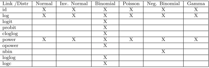
Other links, different from the canonical ones, are possible. However, not all combinations of family and link make sense. Table 2 reports the feasible combinations.

Table 2: Feasible family-link combinations

Link /Distr Normal Inv. Normal Binomial Poisson Neg. Binomial Gamma

id X X X X X X

log X X X X X X

logit X

probit X

cloglog X

power X X X X X X

opower X

nbin X

loglog X

logc X

[image:6.595.136.478.477.589.2]

(7)

treatment can be heteroskedastic. Thus, the variance will vary with the mean which, in turn, varies with explanatory variables.

The GLM is a quasi-maximum likelihood, QML, estimator andβ is obtained by maximizing the following log-likelihood,

l(β)≡ N

X

i=1

li(β)≡ N

X

i=1

logf(Ti;β) = N

X

i=1

logc(Ti, φ) +

Tiθi−a(θi)

φ

(6)

forTi independently distributed.

Being the GPS the conditional density of the treatment received given the covariates, we can compute the GPS by using the exponential density function evaluated at ˆβ, given the covariates

R=r(T, X) =f( ˆβ)

wheref is according to (3). Put another way, the GPS coincides with the vector of the likelihood evaluated at ˆβ,L( ˆβ), whereL( ˆβ) =exp(l( ˆβ)).

However, wheneverT is discrete or fractional a clarification is in order. In these cases the ML in (6) is replaced by the Bernoulli-QML, as in (7)

lB

(β)≡ N

X

i=1

lB i (β) =

N

X

i=1

Tilog[F(Ti;β)] + (1−Ti)log[1−F(Ti;β)] (7)

IfT is binary and (7) is estimated by setting Binomial as family and logit (or probit) as link, equation (7) reproduces exactly the case of binary treatment. In this case the probability of being assigned to treatment, i.e. the pscore, is

F(T = 1) which is the cumulated logit (or probit) evaluated at ˆbeta′XforT = 1. By definition, this is not the cumulated logit (or probit) evaluated at the actual level of the treatment received, which can be either 0 or 1. Starting from this consideration we extend this argument from the binary to the fractional case. Since a great part of the empirical literature has come across the necessity to estimate a dose-response function with fractional treatment data (Fryges and Wagner, 2008; Fryges, 2009 ) we reckon this case to deserve special attention. For this reason we will treat it in more details in the following subsection.

3.1 Flogit or fractional treatment data, a case of particular

interest

(8)

the effect of any particular covariate in Xi cannot be constant over its range.

Augmenting the model with non-linear functions ofXi does not overcome the

problem as the values from an OLS regression can never be guaranteed to lie in the unit interval.

The common practice of regressing the log-odds ratio, i.e. log[T /(1−T)] in the linear regression instead ofT, generates problems whenever any observation

Ti takes on the values 0 or 1 with positive probability. As a practice, in this

situation when Ti are proportions from fixed number of groups with known

group size, the extreme values are adjusted before taking the transformation. However, not always the fractionTi is a proportion from a discrete group size.

In addition, if a large percentage is at the extremes the adjustment mechanism is at least debatable. Papke and Wooldridge sidestep these problems specifying a class of functional forms forE(T|X) and show how to estimate the parameters using Bernoulli-QML, estimator of β, namely the GLM. In particular, they assume that, for alli

E(Ti|Xi) =F(β′Xi) (8)

whereF(.) is typically a logit or probit function, from here the name of flogit estimator.5

Analogously to the binary case, the estimation procedure defines the Bernoulli log-likelihood function as:

li(β)≡Tilog[F(β′Xi)] + (1−Ti)log[1−F(β′Xi)]

and maximizes the sum of li(β) over all N using the GLM. Being the GPS

the probability of the actual, i.e. the observed, treatment received,LB

i (β) does

not coincide with the GPS6_{. [1}₋_F₍_β′_X

i)] attains the probability of receiving

T = 1−t, which is not the actual treatment, i.e. the observed one, but its complement. Hence, it must not enter the gpscore. The estimated GPS based on the Bernoulli log-likelihood function in (5) is:

Ri=F( ˆβ′Xi) ∀i

In this respect, the GPS and the pscore are computable exactly in the same way, whenever the likelihood is Bernoulli.

Therefore, as a general rule we can state that using the GLM in the first step of the dose-response function, to retrieve the GPS one must:

• takeL( ˆβ) whenever the QML is not Bernoulli;

• take F( ˆβ′_X

i) whenever the QML is a Bernoulli-QML, where F(.) is the

probability of succeeding, i.e. of being assigned to treatment t. That is exactly what our programs implement automatically7_.

5_{Notice that in the notation of (4)}_F ₌_g−1 _{for instance, if}_g₍_._{) is the log-odds or logit}

transformation, g(µ) =log[µ/(1−µ)], F = exp(µ)/[1 +exp(µ)] that isF = Λ, the logit distribution.

6

See Wooldridge (2002) pp. 659- 664.

7_{The authors wish to thank K. Hirano for having helped them on this point in a private}

conversation. Differently from our approach in a Bernoulli-QML Fryges and Wagner (2008) and Fryges (2009) takeLB

(9)

4 The Estimation Algorithm

The implementation method can be broken down into three steps. In the first step the program gpscore2.ado estimates the GPS and tests the balancing properties, for any family and link set. In the second step, the conditional expectation of the outcome is estimated as a function of the treatment levelT

and the GPS R, γ(t, r) = E[Y|T = t, R = r]. Finally, in the third step the dose-response functions, ψ(t) = E[γ(t, r(t, X))], is estimated by averaging the estimated conditional expectation, ˆγ(t, r(t, X)), over the GPS at each level of the treatment the user is interested in.

In detail, the first step is implemented as follows:

1. Estimate the parametersθandφof the selected conditional distribution of the treatment given the covariates. Indeed, the distribution ofT is chosen from the exponential family through the family and link option.

2. If the family selected is Normal assess the validity of the assumed Normal distribution model by one of the following, user-specified goodness-of-fit tests: the Kolmogorov-Sminorv, the Shapiro-Francia, the Shapiro-Wilk,or the STATA Skewness and kurtosis test for normality. The user can skip the test through thef lag b(2) option. If the Normal distribution model is statistically disapproved, inform the user that the assumption of Normality is not satisfied. The user is invited to use a different family and link option or a different transformation of the treatment variable.

3. Estimate the GPS as

ˆ

Ri=r(T, X) =c(T,φˆ)exp

(

Tθˆ−a(ˆθ) ˆ

φ )

where ˆθ and ˆφare the estimated parameters in step 1.

4. Test the balancing property and inform the user whether and to what extent the balancing property is supported by the data. Following Hi-rano and Imbens (2004), the programgpscore2.ado tests for balancing of covariates according to the following scheme:

a. Divide the sample in k groups according to an user-specified rule, which should be defined on the basis of the sample distribution of the treatment variable;

b. In the first group, k = 1, compute the GPS at the user-specified representative point. For instance, compute the median of the group and evaluate the GPS for each individual in the sample by setting

t=median of the group;8

c. Take the GPS obtained in the previous point and divide it intonq

sub-intervals defined by its quantiles of orderj/nq, j= 1, . . . , nq−1. Let us call these sub-intervals as blocks;

(10)

d. Within each block, compare individuals who aretreated, i.e. belong-ing to groupk(according to stepa), with individuals who are in the same block but belong to another group. Specifically, within each block calculate the mean difference of each covariate between units belonging to groupkand units not belonging to group k;

e. Combine thenq mean differences, calculated in step [d] by using a weighted average, with weights given by the number of observations in each GPS block;

f. Go to step [b], setk= 2 and go through [b−e];

For each group tests statistics (the t-student statistics or the Bayesian-factor) are calculated and shown in the results window. Finally, the most extreme value of the test statistics (the highest absolute value of the t-student statistics, or the lowest value of the Bayes-factors) is compared with reference values, and the user is informed on to what extent the balancing property is supported by the data. If adjustment for the GPS properly balances the covariates, we would expect all differences to be statistcally not significant.

Notice that for binary treatments, although the GPS is correctly calculated, the dose-response function boils down to a point rather than a curve. For this standard case we refer the user topscore.adoby Becker and Ichino (2002) and topsmatch2.adoby Leuven and Sianesi (2003).9

In the second stage, the conditional expectation for the outcome Yi, given

Ti and Ri, is modelled as a flexible function of its two arguments. We use

polynomial approximations of order not higher than three. Specifically, the most complex model we consider is:

ϕ(E[Yi|Ti, Ri]) = λ(Ti, Ri;α)

= α0+α1Ti+α2Ti2+α3Ti3+α4Ri+α5R2i +α6R3i +α7TiRi

whereϕ(.) is a function that relates the predictor,λ(Ti, Ri;α), to the conditional

expectationE[Yi|Ti, Ri].

The last step consists of averaging the estimated regression function over the score function evaluated at the desired level of the treatment. Specifically, in order to obtain an estimate of the entire dose-response function the program estimates the average potential outcome for each level of the treatment one is interested in, by applying the empirical counterpart of equations (1) and (2), that is:

d E[Y(t)] = 1

N

X

i=1

b

γ(t,br(t, Xi)) =

1

N

X

i=1

ϕ−1(λb(t,br(t, Xi);αb))

Briefly, the programdoseresponse2.adoestimates the dose-response func-tion according to the following algorithm:

9

When the family is binomial the balancing mechanism is slightly different. Indeed, in this case the GPS is independent oft, beingr(t, x) =F(β′_x_{). Therefore, going through step [}_b_],

(11)

1. Estimate the GPS (according to the family and link specified by the user) through the GLM approach, check the normality, if required, and test the balancing property by using the routinegpscore2.ado.

2. Estimate the conditional expectation of the outcome, given the treatment and the GPS, by calling the routinedoseresponse_model.ado.

3. Estimate the average potential outcome for each level of the treatment the user is interested in.

4. Estimate the standard errors of the dose-response function via bootstrap-ping10_.

5. Plot of the estimated dose-response function and, if requested, its confi-dence intervals.

5 Syntax

gpscore varlist weight if in , t(varname) gpscore(newvarname) predict(newvarname) sigma(newvarname) cutpoints(varname) index(string) nq gps(#) family(string) link(string)

t transf(transformation) normal test(test) norm level(#)

test varlist(varlist) test(type) flag b(#) opt nb(string)

opt b(varname) detail

doseresponse model varlist (min=2 max=2) weight if in , outcome(varname) cmd(regression cmd) reg type t(string) reg type gps(string) interaction(#)

doseresponse2 varlist weight if in , outcome(varname) t(varname) gpscore(newvarname) predict(newvarname)

sigma(newvarname) cutpoints(varname) index(string) nq gps(#) dose response(newvarlist) family(string) link(string)

t transf(transformation) normal test(test) norm level(#)

test varlist(varlist) test(type) flag(#) cmd(regression cmd)

reg type t(string) reg type gps(string) interaction(#)

t points(vector) npoints(#) delta(#) bootstrap(string)

filename(filename) boot reps(#) analysis(string)

10_{As in dose-response.ado when bootstrapped standard errors are required, the bootstrap}

(12)

analysis level(#) graph(filename) flag b(#) opt nb(string)

opt b(varname) detail

Note that in the commands gpscore2 and doseresponse2 the argument

varlist represents the control variables, which are used to estimate the GPS. In the commanddoseresponse_model,varlist only consistes of two variables: the treatment variable and the GPS.

6 Option

The doseresponse2 options include all the doseresponse options plus some others strictly related to the GLM estimator. In what follows will be given only a description of the options related todoseresponse2 command, because they include all the options for both gpscore2and the doseresponse_model command. However, for each option it is reported in brackets what command each option is referred to.

6.1 Compulsory Options

outcome(varname) specifies that varname is the outcome variable of the program. [doseresponse2]

t(varname) specifies that varname is the treatment variable [gpscore2 anddoseresponse2].

gpscore(newvarname)asks users to specify the variable name for the esti-mated GPS.[gpscore2]

predict(newvarname) creates a newvar to hold the maximum likelihood estimate of the conditional standard error for the treatment given the covari-ates. [gpscore2]

sigma(newvarname)creates a newvar containing the GLM estimate of the conditional standard error of the treatment given the covariates, obtained from Pearson residuals.11

[gpscore2]

cutpoints(varname)divides the set of the potential treatment values, T, according to the sample distribution of the treatment variable cutting at the

varnamequantiles. [gpscore2]

index(string)specifies the representative point of the treatment variable at which the GPS has to be evaluated within each treatment interval. The argu-mentstringidentifies either the mean (string=mean) or a percentile (string=

11

(13)

p1,...,p100) of the treatment.[gpscore2]

nq gps(#) specifies that the values of the GPS evaluated at representa-tive point index(string) of each treatment interval have to be divided into #(#∈ {1, . . . ,100}) intervals, defined by the quantiles of the GPS evaluated at representative pointindex(string).[gpscore2]

family(string) specifies the distribution family name of the treated vari-able. [gpscore2anddoseresponse2]

link(string)specifies the link function for the treated variable. The default is the canonical link for the family() specified.12 _[gpscore2_and_{doseresponse2]}

dose response(newvarlist) asks users to specify the variable name(s) for the estimated dose-response function(s). [doseresponse2]

6.2 Uncompulsory Options

t transf(transformation)allows users to specify the transformation of the treatment variable being to use in estimating the GPS. The default trans-formation is the identity function. While the supported transtrans-formations are: the logarithmic transformation,t_transf(ln); the zero-skewness log transfor-mation,t_transf(lnskew0); the Box-Cox transformation,t_transf(boxcox) and the zero-skewness Box-Cox transformation,t transf(bcskew0). The Box-Cox transformation finds the maximum likelihood estimates of the parameters of the Box-Cox transform regressing the treatment variablet(varname) on the control variables listed in the input varlist.13 _[gpscore2]

normal test(test) allows users to specify the goodness-of-fit test that gp-score will perform to assess the validity of the assumed Normal distribution model for the treatment conditional on the covariates. By default, gpscore performs the Kolmogorov-Smirnov test. Possible alternatives are: the Shapiro-Francia test for normality,normal_test(sfrancia); the Shapiro-Wilk test for normality, normal_test(swilk); and the STATA Skewness and kurtosis test for normality,normal_test(sktest). [gpscore2]

12

For the list of all the possible family-link combination see table (2).

13_{The problem is whether the treatment variable takes zero value. In such a case, the}

program continues, forcing a transformation of the treatment variable to take a suitable value. Specifically, we assume thatln(0) = 0, andt transf(0) =−1/λifλ >0, andt transf(0) =

(14)

norm level(#)allows to set the significance level of the goodness-of-fit test for normality. The default is 0.05. [gpscore2]

test varlist(varlist)specifies that the extent of covariate balancing has to be inspected for each variable in varlist. The default test varlist consists in the variables The order of magnitude interpretations of the Bayes Factor we apply were proposed by Jeffreys (1961). Used to estimate the GPS. This op-tion is useful when there are categorical variables among the covariates. The command gpscore, which is a regression-like command, requires that categorical variables are expanded into indicator (also called dummy) variable sets and that one dummy-variable set is dropped in estimating the GPS. However, the bal-ancing test should be also performed on the omitted group. This can be done by using the option test_varlist(varlist) and by listing in varlist all the variables, included the complete set of indicator variables for each categorical covariate. [gpscore2]

test(type)allows users to specify whether the balancing property has to be tested using either a standard two-sides t-test (the default) or a Bayes-factor based method test(Bayes factor). The program informs the user if there is some evidence that the balancing property is satisfied. Recall that the test is performed for each single variable in test varlist(varlist) and for each treatment interval. Specifically, let p be the number of control variables in test varlist(varlist), and let K be the number of the treatment intervals. We first calculate p×K values of the test statistic; then we select the worst value (the highestt-value in modulus, or the lowest Bayes factor) and compare it with standard values. [gpscore2]

flag b(#)skips either balancing or normal test or both, takes as arguments 0; 1; 2. If not specified in the commands the program estimates the GPS per-forming both the balancing and the normal test. While if flag b(0) it skips both the balancing and the normal test; ifflag b(1)it skips the balancing test; itflag b(2)it skips the normal test. [gpscore2]

cmd(regression cmd) defines the regression command to be used for esti-mating the conditional expectation of the outcome given the treatment and the GPS. The defaultcmdfor the outcome variable islogitwhen there are two dis-tinct values, mlogit when there are 3−5 values, and regress otherwise. The supported regression commands are: logit, probit, mlogit, mprobit, ologit, opro-bit, and regress. [doseresponse_model]

reg type t(type)defines the maximum power of the treatment variable in the polynomial function used to approximate the predictor for the conditional expectation of the outcome given the treatment and the GPS. The defaulttype

(15)

reg type gps(type) defines the maximum power of the estimated GPS in the polynomial function used to approximate the predictor for the conditional expectation of the outcome given the treatment and the GPS. The defaulttypeis

linear, meaning that the predictorλ(T,Rˆ;α) is a linear function of the estimated GPS. Alternatively,typemay bequadratic, or cubic. [doseresponse_model]

interaction(#) specifies whether the model for the conditional expecta-tion of the outcome given the treatment and the GPS has the interacexpecta-tion be-tween treatment and GPS. The default (#) is 1, meaning that the interaction is included. [doseresponse_model]

tpoints(vector) specifies that doseresponse2 estimates the average po-tential outcome for each level of the treatment in vector. By default, the doseresponse2 creates a vector with ith element equals to the ith observed treatment value. This option can not be used along with the optionnpoints(#) (see below). [doseresponse2]

npoints(#)specifies that doseresponse2estimates the average potential outcome for each level of the treatment belonging to a set of evenly spaced val-uest0, t1, ..., t#, that cover the range of the observed treatment. This option can not be used along with the optiontpoints(#)(see above). [doseresponse2]

delta(#) specifies that doseresponse also estimates the treatment effect function considering a #-treatment gap, which is defined as ψ(t+ #)−ψ(t). The default # is 0, meaning that [doseresponse2] only estimates the dose-response function,ψ(t).

filename(filename) specifies that the treatment levels specified through either the option tpoints(vector) or the option npoints(#), the estimated dose-response function and, eventually, the estimated treatment effect function along with their standard errors (if calculated) are stored to a new file called

f ilename. [doseresponse2]

bootstrap(string) specifies to use bootstrap methods to derive standard errors and confidence intervals. By default, doseresponse does not apply boot-strap techniques. In such a case, no standard error is calculated. In order to activate this option,string should be set toyes. [doseresponse2]

boot reps(#) specifies the number of bootstrap replications to be per-formed. The default isboot reps(50). This option produces any effect only if the bootstrap option is switched on. [doseresponse2]

(16)

dose-response function(s). In order to plot confidence intervals,string has to be set toyes. If the user typesanalysis(no), no plot is shown. [doseresponse2]

analysis level(#) allows the user to set the confidence level # of the confidence intervals. The default confidence level is 0.95.

graph(filename)allows users to store the plots of the estimated dose-response function and the estimated treatment effects to a new file called f ilename. When the outcome variable is categorical,doseresponsecreates a new file for each categoryiof the outcome variable, and names itf ilename i.

opt nb(string) negative binomial dispersion parameter. In the GLM ap-proach you specifyfam(nb #k)where #kis specified through the optionopt nb. The GLM then searches for #k that results in the deviance-based disper-sion being 1. Instead, nbreg finds the ML estimate of #k. [gpscore and doseresponse]

opt b(varname) name of the variable which contains the number of bino-mial trials. [gpscoreanddoseresponse]

detail displays more detailed output. Specifically, this option allows the user to specify that gpscore2 shows the results of the goodness-of-fit test for normality, and some summary statistics of the distribution of the GPS evaluated at the representative point of each treatment interval, and the results of the balancing test within each treatment interval. When this option is specified for doseresponse2, the results of the regression of the outcome on the treatment and the GPS are also shown. [gpscoreanddoseresponse]

7 Stata output

We illustrate the details of our programs using the dataset collected by Imbens et al (2001). In particular, the choice of the dataset has been motivated by the need of comparison with others authors. The aim of the original exercise was to estimate the effect of the prize amount on subsequent labour earnings, “year6”. Being our econometric exercise simply motivated by the need of showing the functioning of the programs we have considered different treatment variables, different from “prize”, that allow us to use different family functions. In par-ticular, the flogit case has been implemented by using the treatment variable “fraction” which is obtained by normalizing the variable “prize” with respect to its highest value in the sample. Accordingly, the results of thegpscore2.ado and of the doseresponse2.ado are shown hereafter. To show the estimation with poisson count data we have used as a treatment variable “edu”, given by the sum of “ownhs” and “owncoll”, namely the years of high school plus the years of college, which, to a certain extent, can be regarded as a count variable. This exercise approximates a return to schooling estimation.

(17)

7.1 Flogit gpscore output

In this case, the treatment variable is “fraction”, which by construction takes on values in the unit interval. The code is implemented by setting the cut points as to divide the sample into three groups contained in the variable cut. The link function is the canonical one, logit. However, other links are admissible according to table 2. The output looks like as follows:

---use "LotteryDataSet", clear

egen max_p=max(prize)

. gen fraction= prize/max_p

. qui gen cut1 = 23/max_p if fraction<=23/max_p

. qui replace cut1 = 80/max_p if fraction>23/max_p & fraction<=80/max_p . qui replace cut1 = 485/max_p if fraction >80/max_p

. gpscore2 male ownhs owncoll tixbot workthen yearw yearm1 yearm2, /// > t(fraction) gpscore(gpscore) ///

> predict(y_hat_ns) sigma(sd_ns) cutpoints(cut1) index(mean) /// > nq_gps(5) family(binomial) link(logit) det

Generalized Propensity Score

****************************************************** Algorithm to estimate the generalized propensity score ******************************************************

Estimation of the propensity score

The treatment is fraction

T

---Percentiles Smallest

1% .0103137 .0023495 5% .0202446 .0023495

10% .0231977 .0103137 Obs 237 25% .0351369 .0110477 Sum of Wgt. 237

50% .0654881 Mean .1138546 Largest Std. Dev. .127485 75% .1299367 .5571485

90% .270282 .629324 Variance .0162524 95% .3482539 .6669279 Skewness 2.888956 99% .629324 1 Kurtosis 15.08626 note: T has non-integer values

Generalized linear models No. of obs = 237 Optimization : ML Residual df = 228 Scale parameter = 1 Deviance = 25.91237504 (1/df) Deviance = .1136508 Pearson = 29.27315861 (1/df) Pearson = .128391

Variance function: V(u) = u*(1-u/1) [Binomial] Link function : g(u) = ln(u/(1-u)) [Logit]

(18)

Log pseudolikelihood = -62.53528122 BIC = -1220.805

---| Robust

T | Coef. Std. Err. z P>|z| [95% Conf. Interval] ---+---male | .6402121 .1694826 3.78 0.000 .3080323 .9723918 ownhs | -.1515907 .1086591 -1.40 0.163 -.3645586 .0613773 owncoll | .0401978 .0431132 0.93 0.351 -.0443026 .1246982 tixbot | .0202427 .0249659 0.81 0.417 -.0286895 .0691749 workthen | .1558366 .2139876 0.73 0.466 -.2635714 .5752446 yearw | -.0169543 .0603052 -0.28 0.779 -.1351503 .1012416 yearm1 | -.0055257 .0131275 -0.42 0.674 -.0312552 .0202037 yearm2 | .0089422 .0134262 0.67 0.505 -.0173726 .035257 _cons | -2.146518 .5413156 -3.97 0.000 -3.207477 -1.085559 ---robust standard errors reported

Estimated generalized propensity score

1% .0556678 .0537445 5% .0600808 .0547833

10% .0659206 .0556678 Obs 237 25% .0749973 .0563906 Sum of Wgt. 237

90% .1541515 .2175611 Variance .0015032 95% .167948 .2198188 Skewness .2804054 99% .2175611 .2256652 Kurtosis 2.511468

******************************************** End of the algorithm to estimate the gpscore ********************************************

****************************************************************************** The set of the potential treatment values is divided into 3 intervals

The values of the gpscore evaluated at the representative point of each treatment interval are divided into 5 intervals

******************************************************************************

*********************************************************** Summary statistics of the distribution of the GPS evaluated at the representative point of each treatment interval ***********************************************************

Variable | Obs Mean Std. Dev. Min Max ---+---gps_1 | 237 .1138546 .0387714 .0537445 .2256652

(19)

************************************************************************************ Test that the conditional mean of the pre-treatment variables given the generalized propensity score is not different between units who belong to a particular treatment interval and units who belong to all other treatment intervals

************************************************************************************

Treatment Interval No 1 - [.0023494709748775, .0474060922861099]

Mean Standard

Difference Deviation t-value

male .07032 .03214 2.1881

ownhs .27061 .13368 2.0244

owncoll .14939 .21863 .6833

tixbot .09136 .43645 .20931

workthen -.01029 .05015 -.20523

yearw .15477 .18022 .85879

yearm1 1.4991 1.7217 .8707

yearm2 1.823 1.5597 1.1688

Treatment Interval No 2 - [.0476247407495975, .1631902456283569]

Mean Standard

male -.06435 .02183 -2.9477

ownhs -.13305 .13008 -1.0228

owncoll -.18433 .19743 -.93368

tixbot -.48247 .38721 -1.246

workthen -.00199 .04998 -.0398

yearw -.33553 .1666 -2.014

yearm1 .07426 1.6071 .04621

yearm2 -.09833 1.4601 -.06734

Treatment Interval No 3 - [.1711813360452652, 1]

Mean Standard

male -.01669 .03175 -.52566

ownhs .19524 .17768 1.0988

(20)

tixbot .47912 .50744 .94421

workthen -.05865 .07293 -.80421

yearw .23415 .22407 1.045

yearm1 -.70637 1.966 -.35929

yearm2 -1.1814 1.7682 -.66816

According to a standard two-sided t test:

Decisive evidence against the balancing property

The balancing property is satisfied at a level lower than 0.01

---7.2

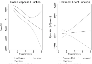
Flogit doseresponse output

Thegpscore2command is replaced by the doseresponse2and additional op-tions are added. Specifically, the matrixtp1contains the value of the treatment we are interested in.

. egen max_p=max(prize) . gen fraction= prize/max_p

. qui gen cut1 = 23/max_p if fraction<=23/max_p

. qui replace cut1 = 80/max_p if fraction>23/max_p & fraction<=80/max_p . qui replace cut1 = 485/max_p if fraction >80/max_p

. mat def tp1 = (0.10\0.20\0.30\0.40\0.50\0.60\0.70\0.80)

. doseresponse2 male ownhs owncoll tixbot workthen yearw yearm1 yearm2, /// > t(fraction) gpscore(gpscore) > predict(y_hat_ns) sigma(sd_ns) cutpoints(cut1)/// > index(mean) nq_gps(5) family(binomial) link(logit) outcome(year6)///

> dose_response(dose_response) tpoints(tp1) delta(0.1) reg_type_t(quadratic)///

> reg_type_gps(quadratic) interaction(1) filename("output_bin") graph("graphoutputbin")/// > bootstrap(yes) boot_reps(10) analysis(yes) det///

******************************************** ESTIMATE OF THE GENERALIZED PROPENSITY SCORE ********************************************

(output omitted)

The outcome variable ´´year6´´ is a continuous variable

The regression model is: Y = T + T^2 + GPS + GPS^2 + T*GPS

(21)

[image:21.595.158.517.340.591.2]

---Bootstrapping of the standard errors ...

The program is drawing graphs of the output This operation may take a while

(file graphoutputbin.gph saved)

End of the Algorithm

---−30000

−20000

−10000

0

10000

E[year6(t)]

0 .2 .4 .6 .8

Treatment level

Dose Response Low bound

Upper bound

Confidence Bounds at .95 % level Dose response function = Linear prediction

Dose Response Function

−10000

−5000

0

5000

10000

E[year6(t+.1)]−E[year6(t)]

0 .2 .4 .6 .8

Treatment level

Treatment Effect Low bound

Upper bound

Treatment Effect Function

(22)

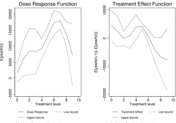
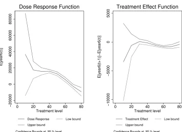
7.3 Gpscore2 and Doseresponse2 for other family functions

In this subsection we report the results for the poisson and gamma distribution with thelog as canonical link funciton.

. gen edu=owncoll+ownhs

. qui gen cut3 = 3 if edu<=3

. qui replace cut3 = 6 if edu>3 & edu<=6 . qui replace cut3 = 9 if edu >6

. mat def tp3 = (0\1\2\3\4\5\6\7\8\9)

. doseresponse2 male workthen yearw yearm1 yearm2, /// > t(edu) gpscore(nostro) ///

> predict(y_hat_ns) sigma(sd_ns) cutpoints(cut3) index(p50) ///

> nq_gps(5) family(poisson) link(log) outcome(year6) dose_response(dose_response) /// > tpoints(tp3) delta(1) reg_type_t(quadratic) reg_type_gps(quadratic) interaction(1) ///

> filename("output_poi") graph("graph_output_poi.eps") bootstrap(yes) boot_reps(10) analysis(yes) det

The treatment is edu

T

1% 0 0 5% 0 0

10% 2 0 Obs 237 25% 4 0 Sum of Wgt. 237

50% 5 Mean 4.970464 Largest Std. Dev. 2.190884 75% 6 8

90% 8 8 Variance 4.799971 95% 8 8 Skewness -.3475038 99% 8 9 Kurtosis 2.762504

Generalized linear models No. of obs = 237 Optimization : ML Residual df = 231 Scale parameter = 1 Deviance = 276.8620777 (1/df) Deviance = 1.198537 Pearson = 219.9190964 (1/df) Pearson = .9520307

Variance function: V(u) = u [Poisson] Link function : g(u) = ln(u) [Log]

(23)

Log pseudolikelihood = -525.4051853 BIC = -986.2598

---| Robust

1% .0060528 .0051862 5% .0158642 .0057593

10% .0435343 .0060528 Obs 237 25% .089226 .0080229 Sum of Wgt. 237

90% .1892501 .1951088 Variance .0030574 95% .1947896 .1953658 Skewness -.8060932 99% .1951088 .2002115 Kurtosis 2.403019

******************************************************************************

(24)

interval and units who belong to all other treatment intervals

************************************************************************************

Treatment Interval No 1 - [0, 3] Mean Standard

male -.06215 .09852 -.63091

workthen -.01101 .01395 -.78881

yearw -.32768 .2437 -1.3446

yearm1 3.4755 2.53 1.3737

yearm2 3.0207 2.5869 1.1677

male .00742 .06118 .12127

workthen .00218 .02025 .10753

yearw -.22962 .138 -1.6639

yearm1 -1.5632 1.2437 -1.2569

yearm2 -1.221 1.3341 -.91525

male .02225 .07089 .31384

workthen -.01708 .04406 -.38773

yearw .12469 .16353 .76246

yearm1 1.7796 1.3134 1.3549

yearm2 1.3032 1.439 .90563

According to a standard two-sided t test: Moderate evidence against the balancing property The balancing property is satisfied at level 0.05 The outcome variable ´´year6´´ is a continuous variable The regression model is: Y = T + T^2 + GPS + GPS^2 + T*GPS

(25)

[image:25.595.160.517.340.590.2]

(file graphoutputpoi.eps saved)

---−5000

0

5000

10000

15000

20000

E[year6(t)]

0 2 4 6 8 10

Treatment level

Upper bound

−20000

−10000

0

10000

E[year6(t+1)]−E[year6(t)]

0 2 4 6 8 10

Treatment level

Upper bound

(26)

. qui gen cut2 = 35 if agew<=35

. qui replace cut2 = 47 if agew>35 & agew<=59 . qui replace cut2 = 59 if agew >59

. mat def tp2 = (10\20\30\40\50\60\70\80)

. doseresponse2 male ownhs owncoll tixbot workthen yearw yearm1 yearm2, /// > t(agew) gpscore(gpscore) ///

> predict(y_hat) sigma(sd_ns) cutpoints(cut2) index(p50) ///

> nq_gps(5) family(gamma) link(log) outcome(year6) dose_response(dose_response) /// > tpoints(tp2) delta(1) reg_type_t(quadratic) reg_type_gps(quadratic) interaction(1) /// > filename("output_gam") graph("graph_output_gam.eps") ///

> bootstrap(yes) boot_reps(10) analysis(yes) det

The treatment is agew

T

1% 24 23 5% 27 24

10% 29 24 Obs 237 25% 36 25 Sum of Wgt. 237

50% 47 Mean 46.94515 Largest Std. Dev. 13.797 75% 56 79

90% 66 80 Variance 190.3571 95% 69 83 Skewness .3402325 99% 80 85 Kurtosis 2.360072

Generalized linear models No. of obs = 237 Optimization : ML Residual df = 228 Scale parameter = .0715905 Deviance = 17.25022412 (1/df) Deviance = .0756589 Pearson = 16.32263484 (1/df) Pearson = .0715905

Variance function: V(u) = u^2 [Gamma] Link function : g(u) = ln(u) [Log]

(27)

---| Robust

T | Coef. Std. Err. z P>|z| [95% Conf. Interval] ---+---male | .0316579 .0393115 0.81 0.421 -.0453912 .1087071 ownhs | -.0462397 .0163188 -2.83 0.005 -.0782239 -.0142554 owncoll | -.0271999 .0119926 -2.27 0.023 -.050705 -.0036948 tixbot | .0034784 .0053921 0.65 0.519 -.0070898 .0140467 workthen | -.1520236 .0530833 -2.86 0.004 -.2560649 -.0479822 yearw | .0080099 .0132164 0.61 0.544 -.0178938 .0339135 yearm1 | -.0081187 .0025995 -3.12 0.002 -.0132136 -.0030237 yearm2 | .0094208 .0026396 3.57 0.000 .0042473 .0145943 _cons | 4.074573 .1030365 39.54 0.000 3.872626 4.276521 ---robust standard errors reported

1% .0042995 .0036313 5% .0049124 .0041178

10% .0052848 .0042995 Obs 237 25% .0063171 .0043183 Sum of Wgt. 237

90% .0114519 .013237 Variance 5.42e-06 95% .0123639 .013259 Skewness .2668858 99% .013237 .0137175 Kurtosis 2.092097

******************************************************************************

(28)

---+---gps_4 | 237 .0052678 .000232 .0045548 .0056592

************************************************************************************ Test that the conditional mean of the pre-treatment variables given the generalized propensity score is not different between units who belong to a particular treatment interval and units who belong to all other treatment intervals

************************************************************************************

Treatment Interval No 1 - [23, 35]

Mean Standard

male .01806 .08032 .22482

ownhs -.15791 .17577 -.89841

owncoll -.17567 .19743 -.88979

tixbot .27769 .52651 .52742

workthen .06134 .059 1.0396

yearw -.17653 .20301 -.86957

yearm1 1.711 2.1394 .79977

yearm2 2.2832 2.0844 1.0954

Mean Standard

male -.01511 .0755 -.20008

ownhs -.22576 .15781 -1.4306

owncoll .00798 .19086 .0418

tixbot -1.1222 .48388 -2.3191

workthen -.11082 .04947 -2.24

yearw .13282 .18882 .70345

yearm1 -3.326 1.9546 -1.7016

yearm2 -2.0772 1.9347 -1.0736

Mean Standard

male -.07167 .07255 -.98797

(29)

owncoll .10901 .20074 .54304

tixbot .14738 .47526 .3101

workthen -.09474 .04986 -1.9001

yearw -.15467 .19021 -.81315

yearm1 -2.5801 2.0016 -1.289

yearm2 -3.2137 1.8802 -1.7092

Mean Standard

male .0267 .09171 .29113

ownhs .05633 .11856 .47506

owncoll .15669 .25743 .60867

tixbot .26623 .59266 .4492

workthen .05137 .04364 1.1772

yearw .03154 .23951 .13167

yearm1 1.7659 2.4575 .71858

yearm2 .70419 2.3628 .29803

According to a standard two-sided t test:

Strong to very strong evidence against the balancing property

The balancing property is satisfied at level 0.01

The outcome variable ´´year6´´ is a continuous variable

The regression model is: Y = T + T^2 + GPS + GPS^2 + T*GPS

Source | SS df MS Number of obs = 202 ---+--- F( 5, 196) = 8.48 Model | 7.3473e+09 5 1.4695e+09 Prob > F = 0.0000 Residual | 3.3978e+10 196 173355070 R-squared = 0.1778 ---+--- Adj R-squared = 0.1568 Total | 4.1325e+10 201 205596471 Root MSE = 13166

(30)

[image:30.595.161.516.299.557.2]

_cons | 940098 738235.5 1.27 0.204 -515806.6 2396003

(note: file graphoutputgam.eps not found) (file graphoutputgam.eps saved)

---−20000

0

20000

40000

60000

80000

E[year6(t)]

0 20 40 60 80

Treatment level

Upper bound

−10000

−5000

0

5000

E[year6(t+1)]−E[year6(t)]

0 20 40 60 80

Treatment level

Upper bound

(31)

8 Conclusions

In recent years there is a growing interest towards the evaluation of policy interventions and more in general towards the estimation of causal effects. In order to accomplish this taskad hoc softwares and programs are needed. The present paper provides two STATA programs implementing the GPS in a very general set up. The programs are very versatile thanks to the introduction of the GLM estimator in the first step of the estimation of the GPS.

Acknowledgements

The paper benefitted from useful comments and suggestions of many people. In particular, the authors wish to gratefully acknowledge E. Battistin, K. Hirano, A. Mattei, J. Wooldridge. The opinions expressed by the authors are their only and do not necessarily reflect the position of the Institute.

9 Bibliography

[1] Becker, S. O., and A. Ichino. 2002.Estimation of average treatment effects based on propensity scores.Stata Journal 2: 358377.

[2] Bia M., and A. Mattei. 2008. A STATA package of the Estimation of the Dose-Response Function through Adjustment for the Generalized Propensity Score. The Stata Journal, 8(3), 354-373.

[3] De Jong P., and G. Z. Heller. 2008.Generalized Linear Models for Insurance Data.Cambridge University press.

[4] Fryges H., and J. Wagner. 2008.Export and productivity growth: first evi-dence from a continuous treatment approach.Review of World Economics, 144(4): 695-722.

[5] Fryges H. 2009.The export-growth relationship: estimating a dose-response function.Applied Economics Letters, 16(18); 1855-1859.

[6] Hausman J.A., and G.K. Leonard. 1997.Superstars in the national basket-ball association: Economic value and policy. Journal of Labor Economics 15, 586-624.

[7] Hirano K., and G.W. Imbens. 2004. The Propensity Score with Continu-ous Treatments. In Applied Bayesian Modeling and Causal Inference from Incomplete-Data Perspective, ed. A. Gelman and X.-L. Meng. Whiley, 73-84.

[8] Imai K., and D.A. Van Dick. 2004. Causal inference with general treat-ment regimes: generalizing the propensity score. Journal of The American Statistical Association, 99: 854-866.

(32)

[10] Imbens G.W., D.B. Rubin, and B. Sacerdote. 2001. Estimating the effect of unearned income on labor supply, earnings, savings and consumption: evidence from a survey of lottery players.American Economic Review, 91: 778-794.

[11] Lechner M.R. 2001.Identification and estimation of causal effects of mul-tiple treatments under the conditional independence assumption, in Econo-metric Evaluation of Labour Market Policies, M. Lechner and F. Pfeiffer eds, Physica, Heidelberg.

[12] Leuven, E., and B. Sianesi. 2003. psmatch2: Stata module to per-form full Mahalanobis and propensity score matching, common sup-port graphing, and covariate imbalance testing. Boston College Depart-ment of Economics, Statistical Software Components. Downloadable from http://ideas.repec.org/c/boc/bocode/s432001.html.

[13] Liu J.L., J.T. Liu, J.K. Hammitt, and S.Y Chou. 1999.The price elasticity of opium in Taiwan, 1914-1942.Journal of Health Economics 18; 795-810.

[14] McCullagh P., and J.A. Nelder. 1989.Generalized Linear Models. Second edition. New York: Chapman and Hall.

[15] Papke L.E. and J.M. Wooldridge. 1996.Econometric Methods for fractional response variables with an application to 401 (K) plan Participation rates. Journal of Applied Econometrics, 11(6): 619-632

[16] Rabe-Hesketh S. and B. Everitt. 2000.A handbook of Statistical Analyses using Stata.Second Eds, Chapman & Hall/Crc. Boca Raton London New York Washington D.C..

[17] Rosenbaum P.R., and D.B. Rubin. 1983.The central role of the propensity score in observational studies for causal inference.Biometrika 70: 41-55.

[18] Rosenbaum P.R., and D.B. Rubin. 1984. Reducing bias in observational studies using classification on the propensity score. Journal of The Ameri-can Statistical Association, 73, 516-24.

[19] Wagner J. 2001.A note on the firm size-export relationship.Small Business Economics 17, 229-337.