Munich Personal RePEc Archive
The sectorial impact of commodity price
shocks in Australia
Vespignani, Joaquin L. and Knop, Stephen J
University of Tasmania
1 January 2014
Online at
https://mpra.ub.uni-muenchen.de/55435/
The sectorial impact of commodity price shocks in Australia
Stephen J. Knop and Joaquin L. Vespignani*
a
University of Tasmania, Tasmanian School of Business and Economics, Australia
Abstract
It is found that commodity price shocks largely affect the mining, construction and manufacturing industries in Australia. However, the financial and insurance sector is found to be relatively unaffected. Mining industry profits and nominal output substantially increase in response to commodity price shocks. Construction output is also found to increase significantly, especially in response to a bulk commodities shock, as a result of increased demand for resource related construction. Increased demand for construction has a positive spillover effect to parts of the manufacturing industry that supply the construction sector with intermediate inputs, such as the non-metallic mineral sub industry. In contrast, other manufacturing sub industries with only tenuous links to the resources sector such as textiles, clothing and other manufacturing, are relatively unresponsive to commodity price shocks.
Keywords: Commodity prices, Commodity Shocks, Australian economy
JEL Codes: E00, E30, F20
**
Corresponding author: Joaquin L. Vespignani; University of Tasmania, School of Economics and Finance, Australia; Tel. No: +61 3 62262825; E-mail address:
1. Introduction
Rapid growth in Asia over the past decade, particularly in China, has had a
substantial impact on the Australian economy. This is well documented in a number of
papers.1 Increased demand for Australia’s natural resources has led to sustained
increases in commodity prices and the terms of trade since 2002. Garton (2008)
explains that these changes in relative prices induce reallocation of resources between
sectors and have boosted real incomes in Australia, stimulating aggregate demand.
However, the benefits of the increase in commodity prices have not been borne
equally by all sectors of the Australian economy. A relatively strong Australian dollar
has resulted in a negative impact on parts of the export sector that have not directly
benefited from the resources boom, such as parts of the manufacturing sector. This
phenomenon is often referred to as ‘Dutch Disease’, and has been discussed at length in
the Australian context. 2
This paper develops a methodology to quantify the impact of commodity prices
on different industries by examining; i) the impact of commodity price shocks in terms
of real and nominal gross value added (GVA) and profits; ii) and examining whether all
commodity price shocks are alike, by disaggregating commodity price indices into bulk
commodities, base metals and rural commodities.3
To find answers to these questions a structural vector autoregressive (SVAR)
model is developed, for the period January 1993 until March 2013.4This paper builds on
existing Australian models that examine shocks to international relative prices such as
1
For example; Dwyer, Gardner and Williams (2011), Kearns and Lowe (2011), Bishop et al. (2013) and Plumb, Kent and Bishop (2013).
2
For recent examples referring to Dutch Disease and the Australian economy see; Mitchell and Bill (2006), Corden (2012) and Lim, Chua and Nguyen (2013).
3
Gross value added is defined as gross output less the intermediate inputs used to produce that output. 4
Dungey and Pagan (2000), Jääskelä and Smith (2011) and Dungey, Fry-Mckibbin and
Linehan (2014), while also integrating the methodology of analysing specific industries,
as in Lawson and Rees (2008) and Vespignani (2013).
The major finding of this study is that commodity price shocks have a
significant positive impact on mining sector profits and nominal GVA. Conversely, real
GVA in the mining sector declines (in the short run) in response to commodity price
shocks. Mines are often run at close to full capacity, and a sudden increase in
commodity prices encourages increased extraction of minerals. In the short term this
requires the use of more intermediate inputs such as labour, resulting in higher cost
production. This can have a negative impact on real GVA in the mining industry in the
short-run. Results also indicate that commodity price shocks increase output in the
construction sector, due to increased demand for resource related construction.
However, manufacturing profits decline significantly in response to commodity price
shocks.
The paper proceeds as follows. Section 2 details the importance of commodity
prices to the Australian economy. Section 3 provides a review of the existing literature.
Section 4 outlines the SVAR methodology and modelling identification assumptions.
Section 5 presents an extended model. Section 6 presents the results of commodity price
shocks on industry variables in terms of impulse responses and variance decomposition.
Section 7 provides a brief robustness analysis. Section 8 concludes.
2. Commodity prices and the Australian economy
Connolly and Orsmond (2011) explain that the floating exchange rate has had a
Australian dollar. Subsequently, increased inflationary pressures have not accompanied
the surge in mining related investment and activity as they did during previous booms.
Commodity prices have also been affected by the substantial change in the
composition of global growth. In particular, the increased importance of China has
resulted in a global demand shift towards commodities.5 Connolly and Orsmond (2011)
outline that the increase in global commodity prices during the 2000s has made mining
more profitable and encouraged a shift in labour, investment and materials into the
mining industry. While the increase in global commodity prices has been broad,
Connolly and Orsmond (2011) highlight that there has been particularly large increases
in the price of steelmaking commodities such as coking coal and iron ore. Over the past
decade, commodity exports have, on average, contributed 55 per cent of total export
values and 11 per cent of Australian GDP.
Figure 1 shows the evolution of the RBA index of commodity prices
disaggregated into rural, base metals and bulk commodities in US dollars from January
1993 to March 2013.
Rural commodities include food products such as lamb, wheat, beef and veal.
Iron ore and coal are both bulk commodities, while base metals refer to metals such as
aluminium, lead and copper. Clearly evident in Figure 1 is the increase in the prices of
bulk commodities and base metals after the onset of the mining boom and their rapid
decline during the GFC. Rural commodity price fluctuations have not been as extreme
over the same time period, though they have still been relatively volatile.
5
3. Literature review
The sectoral impact of commodity prices on the Australian economy is analysed
in a non-SVAR framework by Rayner and Bishop (2013), who use input-output tables
to quantify the links between domestic industries. They conclude that the mining boom
has had a positive impact on sectors that supply inputs to the resources sector, such as
resource related construction and manufacturing. However, the output of industries not
directly related to the resources sector has declined due to a stronger currency and
increased competition for factors of production.
In terms of SVAR studies that analyse industry level data, internationally there
are a number of papers that have examined the impact of commodity prices on specific
industries, with a many of these focusing on oil price shocks. However to date, sectoral
responses to commodity price shocks have not been examined in an Australian SVAR.
Lee and Ni (2002) examine the effects of oil price shocks across 14 different
industries in the United States using an identified VAR model. Their results indicate
that for the majority of industries, oil shocks significantly decrease output.
Many studies focus on the impact of commodity prices on the manufacturing
sector. Jiménez-Rodríguez (2008) find that an oil price shock decreases the level of
manufacturing output across all countries examined. However, results suggest oil price
shocks produce different reactions across sub industries within the manufacturing
industry.
Guidi (2010) analyses the impact of oil price shocks on the performance of both
the manufacturing and service sectors in the United Kingdom. His analysis indicates
that output in the manufacturing sector contracts significantly, and the service sector is
and Sudo (2010) find that oil price shocks have a positive impact, in terms of output, on
oil-intensive industries in Japan.
4. Methodology
A SVAR model is constructed using quarterly data from March 1993 until
March 2013, spanning 81 observations, our sample period coincides with the Reserve
Bank of Australian moves to inflation targeting in 1993.
When estimating a SVAR model for a small open economy it is common to
incorporate two sets of variables; foreign variables representing world economic
conditions and domestic variables that attempt to model the domestic economy.
Following Australian studies such as Dungey and Pagan (2000), Lawson and Rees
(2008), Jääskelä and Smith (2011), Vespignani (2013), a small open economy
assumption is present in the SVAR model. The domestic variables are affected by the
world economy, but by specifying the foreign variables as exogenous, there is no
feedback within a quarter.
4.1 Foreign variables
The purpose of the foreign variables is to model world economic conditions.
While for the majority of the 20th century the United States boasted the world’s largest
economy, in the 21st century, emerging countries such as China have increased their
share of world real GDP significantly. China’s prominence to the Australian economy is
especially important, as they purchase a substantial amount of Australian exports,
particularly commodities. For this reason when modelling international economic
conditions, it is important to take into consideration the changing structure of the global
Figure 2 shows Australia’s largest trading partners in terms of total trade value
from January 1993 until March 2013. China’s increasing importance to the Australian
economy is clear, as is the declining role of the United States.
As a result of the diminishing importance of the United States economy in
contributing to Australian economic outcomes, this study incorporates a weighted
bundle of economies when representing global economic conditions.
There are three exogenous foreign variables; world real gross domestic product
in U.S dollars ( ), a world inflation rate ( ) and a world interest rate
( ).
For this study, proxies of world output, inflation and a world interest rate are
derived from GDP, consumer price index (CPI) and interest rate data from Australia’s
five largest trading partners; China, Japan, the United States, the United Kingdom and
the Euro area.
is an aggregation of quarterly real GDP of Australia’s five largest
trading partners, seasonally adjusted, all measured in United States Dollars. is
constructed by aggregating government policy rates and weighting by their share of
Australian trade. is constructed by aggregating consumer price indices for each
of the five countries, rebasing to a common base year, and weighting by their share of
Australian trade.
4.2 Domestic variables
The second group of variables represents the Australian economy and builds on
the models of Dungey and Pagan (2000), Lawson and Rees (2008), Vespignani (2013)
Consistent with existing Australian SVAR literature (Brischetto and Voss, 1999;
Berkelmans, 2005; Lawson and Rees, 2008; Vespignani, 2013), real Australian
GDP is used as a measure of domestic output. Following Jääskelä and Smith
(2011) and Dungey, Fry-Mckibbin and Linehan (2014), non-farm GDP is used, as farm
GDP can suffer from extreme short-term volatility due to weather effects. In order to
analyse industry specific responses, the variable is defined as Australian GDP
minus the GVA of industry i. This method follows Lawson and Rees (2008) and
Vespignani (2013) and ensures that and sum to total Australian
non-farm GDP when analysing each individual industry. is the real GVA of industry i.
In order to analyse the impact of commodity prices on individual industries
more thoroughly, two subsidiary measures of industrial output are also considered;
industry profits before income tax ( and nominal GVA ( . Each variable
is included in the SVAR model one at a time in place of real GVA
is a measure of relative prices in Australia. The CPI excluding interest and
tax changes of 1999-2000 is used in line with most Australian papers.6The target cash
rate ( ) is included as a measure of the policy reaction function of the central
bank. The trade-weighted index is included as a measure of the real exchange
rate following the majority of Australian SVAR studies.
The SVAR can be expressed by the following structural form (ignoring for
simplicity any constant terms in the model):
(1)
where , is a vector of endogenous variables:
, , , ] (2)
6
See for example, Dungey and Pagan (2000), Berkelmans (2005), Lawson and Rees (2008), Claus, Dungey and Fry (2008), Jääskelä and Smith (2011) and Vespignani (2013). The inflation rate has been
and is a vector of exogenous variables:
] (3)
The vector contains the orthogonal structural disturbances, which are identified by
placing restrictions on the matrix, which are proposed in the following section.
4.3 Identification Restrictions
In line with these international and domestic studies, we impose restrictions only
on the contemporaneous relationships between the variables.
, and are our measures of international economic
conditions. These foreign variables are specified as strictly exogenous, which follows
Jacobs and Rayner (2012) and Vespignani (2013).
Commodity prices are the most exogenous of the domestic variables. It is
assumed that none of the Australian variables can contemporaneously influence world
commodity prices due to the small size of the Australian economy. Australian domestic
variables can influence commodity prices in lags, in line with Dungey, Fry-Mckibbin
and Linehan (2014). is affected contemporaneously by commodity prices,
which is standard across the existing literature. The cash rate does not
contemporaneously affect GDP as monetary policy takes time to influence consumption
and investment decisions.
is contemporaneously affected by commodity prices and Australian GDP.
Fluctuations in commodity prices are likely to influence production decisions in
industries such as mining and manufacturing and consequently impact on industry GVA
in the same quarter. is ordered after as in Lawson and Rees (2008) and
Vespignani (2013). Reasoning for this is that each industry comprises only a small
effects on individual industries in the same quarter. Due to the interrelated nature of
nominal GVA ( , industry profits ( and real GVA we utilise the
same contemporaneous restrictions when each variable is considered.
responds immediately to commodity prices and Australian domestic
output, which is consistent with Brischetto and Voss (1999), Dungey and Pagan (2000),
Berkelmans (2005), and Lawson and Rees (2008). Shocks to commodity prices, such as
the price of oil, would be expected to influence the inflation rate in the same quarter as
firms change their prices quickly in response to the change in price of an important
input. Inflation does not respond to the cash rate contemporaneously as changes in the
cash rate take time to influence consumption and investment decisions, and hence flow
through to prices. Jacobs and Rayner (2012) explain that inflation does not respond
immediately to changes in the trade-weighted index as these changes occur gradually.
There are two common methods of specifying the contemporaneous restrictions
in the domestic cash rate equation. The first method allows contemporaneous
interaction between the cash rate and variables that are deemed to be observable by the
RBA at the time of the policy decision.7 The second involves specifying a Taylor type
monetary policy rule whereby the domestic cash rate responds contemporaneously to
inflation and domestic output.8 In our specification we have chosen the latter approach,
and have allowed the cash rate to respond contemporaneously to commodity prices,
inflation and Australian GDP.9
responds contemporaneously to all variables and is the most endogenous
variable in our system. This is standard in the majority of domestic and international
7
For example, Brischetto and Voss (1999), Berkelmans (2005), Lawson and Rees (2008), Jacobs and Rayner (2012) and Vespignani (2013).
8
For example, Dungey and Pagan (2000, 2009), Claus, Dungey and Fry (2008), Dungey, Fry-Mckibbin and Linehan (2014).
9
literature, as the exchange rate is a variable that trades daily and responds quickly to all
available information. A summary of these identification restrictions is shown in
Equation (4).
[
][
10
]
Given these restrictions the model is over-identified; there is one more zero
restriction than necessary to just identify the model. The likelihood ratio test for over
identification is calculated for each of the permutations of the SVAR considered (profit
and real and nominal GVA of each industry). In all but one case the null hypothesis of
valid over-identification restrictions cannot be rejected at the 10 per cent level,
indicating that the restrictions placed on the model are reasonable.11
Two lags of the exogenous foreign variables affect all domestic variables, and
world GDP also affects the domestic variables contemporaneously. Allowing
contemporaneous interaction between world GDP and the domestic variables is
consistent with Dungey and Pagan (2000), Berkelmans (2005), Lawson and Rees
(2008) and Dungey, Fry-Mckibbin and Linehan (2014) and is supported by the model.12
10
Nominal GVA and industry profits are also considered in place of real GVA, with the same contemporaneous restrictions. However when nominal GVA is considered, real GDP is replaced with nominal GDP. When industry profits are considered, non-farm real GDP remains as an unadjusted variable, rather than subtracting the industry of interest.
11
Statistics are available in Appendix B, Table 4. 12
4.4 Choice of lag length
To select the lag length, the Schwartz Bayesian, Hannan-Quinn and Akaike
information criteria are considered for each industry. For each industry, the Schwartz
and Hannan-Quinn criterion suggest one lag and the Akaike criterion suggests eight lags
with the exception of the construction industry where it indicates seven lags. Including
too many lags risks over parameterising the model, however selecting too few may
result in omitted variable bias. Consequently, a lag length of is selected in line
with Jacobs and Rayner (2012) and Dungey Fry-Mckibbin and Linehan (2014) .
4.5 Tests for stationarity
The Augmented Dicky Fuller (ADF) and Kwiatkowski-Phillips-Schmidt-Shin
(KPSS) tests are conducted to determine whether the variables are stationary. The null
hypothesis of the ADF test is that the variable is non-stationary; the KPSS test has the
opposite null hypothesis, that the variable is stationary. Test statistics are shown in
Table 5, located in Appendix B.
For the majority of the variables, the ADF and KPSS tests suggest that the
variables are non-stationary in levels. Both tests support that the domestic inflation rate
and industry profits are stationary in levels at the 10 per cent level. The statistics for the
ADF and KPSS tests are -6.041 and 0.115 for inflation and -4.624 and 0.072 for
industry profits, respectively.13. Table 5 also shows the results of unit root testing using
the first difference of the variables that are non-stationary in levels. Both ADF and
KPSS tests indicate that these variables are all first difference stationary at the 10 per
cent level of significance.
13
5. Extended model
In this section we consider an extended model, by disaggregating commodity
prices into individual components. Three separate commodity price indices are reported
by the RBA: rural commodities, base metals and bulk commodities.
We specify bulk commodities as the most exogenous variable. Justification for
this is that the majority of the bulk commodities index is made up of coal, which is used
in generating a substantial amount of the world’s supply of electricity. An increase in
bulk commodity prices, and hence in the cost of generating electricity, is likely to have
flow on effects to rural commodity and base metals prices. Base metals are ordered as
the second variable, followed by rural commodities. Rural commodities are ordered
after base metals as metals are used as inputs in a large number of industries.
Different contemporaneous relationships between the commodity price indices
are considered, and the restrictions which are most supported by the model are selected.
To determine the most appropriate restrictions, the criteria of the highest p-value when
testing for valid over-identifying restrictions is employed. The resulting restrictions
( are shown in Equation (5). Similarly to the baseline model
introduced in Section 4, two lags of the exogenous foreign variables enter the model,
and world GDP is allowed to affect the domestic variables contemporaneously. 14
[
][
]
14
Given these restrictions the model is over-identified; there is one more zero
restriction than necessary to just identify the model. The likelihood ratio test for over
identification is calculated for each of the permutations of the SVAR considered (profit
and real and nominal GVA of each industry). In the majority of these tests, the null
hypothesis of valid over-identification restrictions cannot be rejected at the 10 per cent
level, indicating that the restrictions placed on the model are reasonable. 15
6. Results
This section analyses the cumulative impulse responses of industry variables to
commodity price shocks and the variance decomposition of the estimated SVAR.
One per cent shocks are applied to the SVAR model. For the impulse responses
presented in this section, asymptotic standard errors of one standard deviation are used.
Since we are focusing on the industrial impact of commodity price shocks, most of the
analysis within this section centres on the responses of the industry variables to
innovations to commodity price indices. However, in Section 6.5 we also consider
shocks to our domestic variables in order to check the adequacy of the model.
Sensitivity checks are also performed on each of our SVAR models. The presence of
residual heteroskedasticity is rejected in all models at the 10 per cent level, and for the
majority of the models first order serial correlation is not present.16
6.1 Commodity price shocks: All items
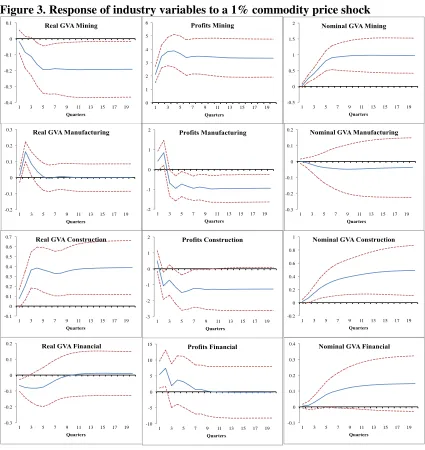
Figure 3 indicates that in general, the impulse responses of real and nominal
GVA and profits respond in a similar fashion. However, two notable exceptions are the
mining and construction industries.
15
Statistics are available in Appendix B, Table 4. 16
A one per cent shock to commodity prices results in a negative response of
mining real GVA that reaches its minimum at 0.2 per cent below the baseline in the fifth
quarter and remains significantly negative from the fourth quarter over the impulse
horizon.
The response of mining profits and nominal GVA provide a stark contrast; both
are significantly positive over the entire impulse horizon, mining profits increase by 2.1
per cent contemporaneously, before peaking at 3.9 per cent in the fourth quarter. These
contrasting results are due to the different way in which real and nominal GVA are
constructed.
Real GVA is a volume measure of production of a particular industry. Topp et
al. (2008) explain that the surge in commodity prices during the past decade
considerably increased the value of output produced by the mining sector, but had little
impact on the volume of output in the short run (measured by real GVA). Furthermore,
increasing commodity prices encourages extraction of ‘more-marginal’ deposits, which
require more intermediate input per unit of output, resulting in higher cost production.
In addition, mines are also usually run at, or close to, full capacity. Consequently output
can only be increased in the short term by using more intermediate inputs such as
labour. Topp et al. (2008) also highlight that there is a significant lead-time associated
in investing in new production capacity (such as new mine sites) and the corresponding
increase in output. Accordingly, an increase in commodity prices does not lead to a
significant increase of real mining GVA in the short term, due to the cost of
intermediate inputs increasing by more than the gross volume of output.
Turning to the construction sector, the response of real and nominal GVA for the
industry is positive. Real GVA peaks at 0.35 per cent in the fourth quarter, and remains
(2014) find that a commodity price shock results in an increase in mining investment,
such as the building of new mine sites. As the construction industry will be involved in
the creation of these new mines, the real GVA of the construction industry is likely to
increase.
In response to a one per cent commodity price shock, manufacturing real GVA
responds positively in the second quarter before declining to baseline in subsequent
periods. Profits increase at first before declining sharply. Commodities are intermediate
inputs in a range of manufacturing sub industries, and a commodity price shock may be
expected to result in a decline in real output in the industry by increasing the costs of
production in certain sub sectors. However, certain manufacturing industries provide a
large amount of inputs for the construction industry, and will face increased demand
following commodity price shocks as the construction sector increases output.
6.2 Commodity price shocks: Bulk commodities
In figure 4, the responses the responses of industry variables to a bulk
commodity shock are shown, these responses remain similar to the responses to an all
items price shock. Industry profits continue to closely follow real GVA with the
exception of the mining and construction industries.
Mining real GVA responds negatively to a one per cent increase in bulk
commodity prices, stabilising at negative 0.08 per cent, and is significantly negative
from period three onwards. As found previously, mining profits and nominal GVA
respond significantly positively over the impulse horizon.
Construction real GVA responds positively to a bulk commodity shock for the
entire impulse horizon, peaking at 0.23 per cent in the third quarter. Increases in the
construction industry is required to build new mine sites. Construction profits increase
by 0.38 per cent contemporaneously before declining. This mixed response is due to the
conflicting impact of a bulk commodity price shock on construction industry profits;
increased demand for resource related construction has a positive impact on industry
profits, while the price of inputs such as steel increases, decreasing profits.
The response of manufacturing real GVA and profits increase initially before
declining, likely due to the contrasting responses within sub sectors. The response of
manufacturing sub industries real GVA to a bulk commodities shock is analysed in the
following section. Similarly to the all items commodity price shock, financial services’
GVA and profits remain unresponsive to a bulk commodity price shock.
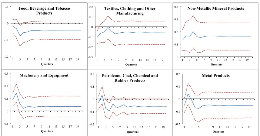
6.2.1 The response of manufacturing sub industries
Since manufacturing is a broad sector, the ABS disaggregates real
manufacturing GVA into eight sub sectors. Six of these sectors are examined.17
In figure 5, the results of these subsectors within the manufacturing industry
provide a better understanding of the response of the entire industry to a bulk
commodity price shock. Some sectors suffer from rising input costs, others benefit from
resource related demand spillovers from other industries such as construction.
Sub industries such as metal products and Food, beverage and tobacco product
manufacturing remain relatively unresponsive to a bulk commodity price shock. The
petroleum, coal, chemical and rubber product sector experiences a reduction in output in
response to a bulk commodity price shock, likely due to increased cost pressures as the
price of inputs such as coal rise.
17
In contrast the non-metallic mineral products reacts positively to a bulk
commodities shock, real GVA increases by 0.17 per cent contemporaneously, peaking
at 0.23 per cent and remains significantly positive over the impulse horizon. This is due
to the construction industry requiring products manufactured by this sub industry. 18
6.3 Commodity price shocks: Base metals
Figure 6 shows the responses of industry variables to a one per cent base metals
shock. A base metal shock has a relatively smaller effect than a bulk commodities
shock, highlighting the increased importance of bulk commodities.
Mining real GVA is unresponsive to a one per cent increase in base metals,
echoing the results in the previous sections; real output in the mining industry does not
increase in the short term following increases in commodity prices, due in part to
capacity constraints.
However, profits and nominal GVA respond positively which can be attributed
to the increase in the value of the outputs of mining industry. This response is smaller in
magnitude than the increase in profits associated with a bulk commodities shock,
underlining the importance of iron ore and coal relative to base metals for the mining
industry. 19Manufacturing output is relatively unresponsive, while profits increase
initially before declining.
Construction real GVA has a negative contemporaneous response of 0.08 per
cent before increasing above the baseline, though not significantly. This is potentially
attributed to the use of base metals as an input by the construction industry; increases in
prices result in an immediate increase in cost pressures, influencing output. However,
18
Over 63 per cent of the non-metallic mineral sectors output was used by the construction industry in 2008/09. See ABS Input-Output tables cat 5209.0 Table 2.
19
increases in base metal prices are also associated with an increase in mining investment,
which increases construction output, so the net effect over the period is negligible.
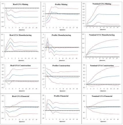
6.4 Commodity price shocks: Rural commodities
This section (figure 7) shows the responses of industry variables to one percent
rural commodity shock. A rural commodity shock has a positive impact on
manufacturing, increasing real GVA by 0.16 per cent in the fourth quarter. A substantial
amount of the intermediate inputs used in the agricultural sector are provided by the
manufacturing industry.20 An increase in rural commodity prices is likely to encourage
increased agricultural production and the demand for intermediate inputs, stimulating
output in the manufacturing industry.
In contrast, manufacturing industry profits increase initially, before falling
below baseline in subsequent periods. This is due to the interrelated nature of the
manufacturing and agricultural sectors; the biggest sub industry in manufacturing (food,
beverage and tobacco product manufacturing) requires a substantial amount of rural
commodities as inputs.21 The manufacturing sector initially experiences increased
demand for their products from the agricultural sector, which increases profits.
However, in the longer term some sub industries’ profits decline due to increased input
costs.
The response of real mining GVA to a one per cent rural commodity shock
peaks at negative 0.2 per cent in the seventh quarter, remaining significantly negative
throughout the impulse horizon. In the model, commodity price shocks result in an
20
In 2008-09 approximately 23 per cent of intermediate inputs in the agricultural industry were provided by the manufacturing industry. See ABS Input-Output tables cat 5209.0 Table 2.
21
exchange rate appreciation.22 Intuitively, this has a negative impact on demand in the
mining industry as commodity exports become relatively more expensive to overseas
buyers.
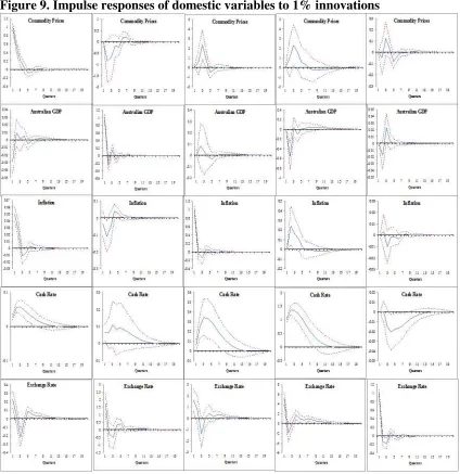
6.5 Shocks to the domestic variables
This section outlines the impulse responses of the baseline model domestic
variables.23 Non-cumulative impulse responses are discussed, in order to make direct
comparisons with a number of Australian SVAR models.24
The responses of the domestic variables to a commodity price shock are
consistent with those presented in Dungey, Fry-Mckibbin and Linehan (2014).
Australian GDP falls in response to a commodity price shock, though the response is
small and only significant in the initial period. Dungey, Fry-Mckibbin and Linehan
(2014) attribute this fall in production to a decline in activity in the non-resources sector
that is not fully compensated for by an increase in production in the resources sector.
Inflation increases contemporaneously in response to rising commodity prices, but
declines in subsequent periods. The decline in the inflation rate is due to an appreciation
of the real exchange rate making imported goods cheaper, and an associated contraction
of the domestic cash rate that reduces inflationary pressures. The cash rate initially
increases before declining as commodity prices and inflation fall.
The real exchange rate originally appreciates in response to commodity price
shocks. In cumulative terms (not shown in this figure) the impact of commodity prices
remains positive even after 2 years. Results are consistent in terms of sign, magnitude
and significance to those observed in Dungey, Fry-Mckibbin and Linehan (2014). The
impact of commodity prices on the exchange rate helps to explain the negative impact
22
See Appendix B, Figure 9 for impulse responses of a commodity price shock on the exchange rate. 23
The model is identical to the baseline model in Section 4, but without an industry variable present. 24
of commodity prices in the mining real GVA observed in figure 3. Following the
standard Mundell and Fleming model with a floating exchange rate and perfect capital
mobility, an appreciation in the domestic currency leads to a reduction in net exports, as
exports became more expensive for foreign economies while imports for the domestic
economy became cheaper.
Figure 9 also shows that the appreciation of the exchange rate as a consequence
of commodity price shocks, occur immediately in the first quarter, while the
transmission from the exchange rate to real output, inflation and monetary reaction
occur after the first quarter. Variance decomposition results show that up to 13% of the
Australian exchange rate variation can be explained by commodity price shocks.
An inflation shock results in a sustained increase in the cash rate that peaks in
the third quarter before slowly returning to the baseline. The exchange rate initially
increases before falling below baseline in the third period. GDP is unresponsive to an
inflation shock.
As expected, GDP decreases in response to a shock to the cash rate. However,
the response of inflation highlights the presence of a ‘price puzzle’, whereby a domestic
cash rate contraction leads to an increase in inflation. The increase in inflation is
short-lived, as the response decreases after the first two periods, moving below the baseline in
period six. The response of inflation to a cash rate shock is comparable to Lawson and
Rees (2008) and Jacobs and Rayner (2012) who find a similar ‘price puzzle’ in their
results. In response to an unanticipated increase in the cash rate, the exchange rate
appreciates initially, before depreciating, consistent with uncovered interest rate parity.
In response to an exchange rate shock the cash rate decreases, as monetary
6.6 Variance decomposition
Variance decomposition provides information on the proportion of the variation
in each of the variables that can be explained by shocks to the other variables within the
model. The variation decomposition for the baseline model is shown below, focusing
only on the results of industry variables to a commodity price shock innovation.
The results in Table 1 highlight the importance of commodities in the mining,
manufacturing and construction industries. In the mining industry shocks to commodity
prices explain only a small amount of variation in real GVA, compared to the large
amount of variation explained in nominal GVA and profits. This result highlights the
muted response of real output, relative to nominal output, in the mining industry to
increases in commodity prices found in previous sections. Commodity prices explain
more of the variation in profits in the mining, manufacturing and construction industries
than in the financial services and insurance sector. This is unsurprising as commodities
are direct inputs into the manufacturing and construction industries, and will likely have
a more significant impact on industry wide profits.
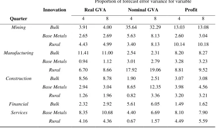
Table 2 shows the results of the variance decomposition for the extended model.
In a similar vein to the impulse response results, bulk commodities shocks explain only
a relatively small amount of the variation in real mining GVA (3.91 per cent after four
quarters), in contrast to the large amount of variation explained in nominal mining GVA
and profits (35.64 and 13.03 per cent after four quarters, respectively). Bulk commodity
shocks explain a larger amount of the variation in the mining, construction and
manufacturing industries relative to financial services.
The results for the construction industry also reaffirm the impulse response
results; rural commodity shocks explain little of the variation in real construction GVA
is tenuous. Base metals explain the most variation in terms of profits (3.98 per cent in
the fourth quarter), due to the impact of base metals on input costs, and bulk
commodities explain the most in terms of real GVA (8.56 per cent in the fourth quarter).
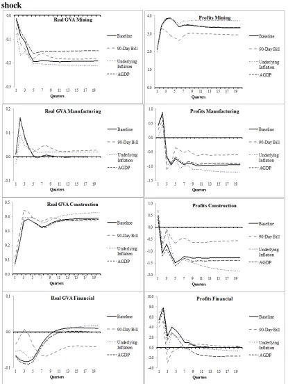
7. Robustness analysis
SVAR systems can be sensitive to the specification of the model. Accordingly,
this section examines a number of alternate specifications to determine the robustness of
our results. Using alternate variables in the baseline model. Figure 8 shows the effect of
estimating the model with the 90-day bill rate, Australian GDP and trimmed mean
inflation as alternative variables.
7.1 Variable specification
To consider the impact that including different variables in the model may have,
the alternate variables in Table 3 are substituted into the baseline model one at a time.
We consider using a different weighting scheme for our exogenous foreign variables, by
weighting the world inflation and interest rate by GDP rather than by trade. The use of
GDP weighting has little impact on our results. The use of Australian GDP instead of
non-farm Australian GDP is also examined, with the results shown in Figure 8. We also
consider using the 90-day bill rate, as this rate closely follows the domestic cash rate
target and more directly reflects the costs that banks pay for short-term funds. Finally,
we incorporate a measure of underlying inflation, as this is used in some previous
studies (Lawson and Rees, 2008; Jacobs and Rayner, 2012; Dungey, Fry-Mckibbin and
Linehan, 2014). There are no discernible changes to our results when substituting
8. Conclusions
The three industries that are most affected by commodity price shocks are the
mining, construction and manufacturing industries. In comparison, the output and
profits of the financial and insurance sector is found to be relatively unaffected.
The results indicate that the value of mining output and industry profits increase
substantially in response to a commodity price shock. Conversely, impulse responses
show that the volume of real mining output responds negatively to a commodity price
shock. This is partly due to rising commodity prices encouraging extraction of more
marginal deposits, which requires more intermediate input per unit of output. These
results are reemphasised in the variance decomposition with commodity price shocks
explaining a substantial amount of variation in the value of mining sector output
(nominal GVA and profits) and little of the real volume of output (real GVA).
The construction and parts of the manufacturing industry are both found to
benefit from demand spillovers from the resources sector. In response to commodity
price shocks, construction output increases significantly as a result of increased demand
for resource related construction. Variance decomposition also shows that commodity
prices explain a significant amount of variation in the output and profits of the
construction industry.
Manufacturing output also increases in response to a commodity price shock,
however profits only increase initially before declining, highlighting increased cost
pressures in manufacturing in the longer term. More generally, analysis of innovations
to each of the three commodity price indices reveals that bulk commodity prices have a
greater impact on industry variables relative to rural commodities and base metals,
Our findings also suggest that the floating exchange rate policy in Australia has helped
significantly to stabilise the economy in the presence of commodity price shocks. 25A
rise in commodity prices substantially increases the value of the Australian currency
which reduces competitiveness of Australian exports. Mining real outputs are materially
affected by the appreciation of the Australian dollar, as this sector exports most of its
production.
References
Berkelmans, L 2005, ‘Credit and Monetary Policy: an Australian SVAR’, Reserve Bank of Australia, Research Discussion Paper, No. 2005–6.
Bishop, J, Kent, C, Plumb, M & Rayner, V 2013, ‘The Resources Boom and The Australian Economy: A Sectoral Analysis’, RBA Bulletin, March, pp. 39–49.
Brischetto, A & Voss, G 1999, ‘A Structural Vector Autoregressive Model of Monetary Policy in Australia’, Reserve Bank of Australia, Research Discussion Paper, 1999–11.
Claus, E, Dungey, M & Fry, R 2008, ‘Monetary Policy in Illiquid Markets: Options for
a Small Open Economy’ Open Economies Review 19,305-336.
Dungey, M, Fry-Mckibbin, R & Linehan, V 2014, ‘Chinese resource demand and the
natural resource supplier’, Applied Economics, 46, 167-178.
Dungey, M & Pagan, A 2000, ‘A structural VAR model of the Australian economy’, The Economic Record 76, 321–42.
Dungey, M & Pagan, A 2009, ‘Extending a SVAR model of the Australian economy’, The Economic Record 85, 1–20.
Dwyer, A, Gardner, G & Williams, T 2011, ‘Global Commodity Markets – Price Volatility and Financialisation’, RBA Bulletin, June, pp. 49–57.
Fukunaga, I, Hirakata, N & Sudo, N 2010, ‘The Effects of Oil Price Changes on the Industry-level Production and Prices in the U.S. and Japan’, NBER Working Paper 15791, National Bureau of Economic Research, Cambridge, MA.
Garton, P 2008, ‘The resources boom and the two-speed economy’, Australian Treasury, Economic Round-up 3, 17-29.
25
Guidi, F 2010 ‘The Economic Effects of Oil Price Shocks on the UK Manufacturing and Services Sectors’, The IUP Journal of Applied Economics 9, 5-34.
Jääskelä, J & Smith, P 2011, ‘Terms of Trade Shocks: What are They and What Do They Do?’, Reserve Bank of Australia, Research Discussion Paper 2011-05.
Jacobs, D & Rayner, V 2012, ‘The Role of Credit Supply in the Australian Economy’, Reserve Bank of Australia, Research Discussion Paper 2012-02.
Jiménez-Rodríguez, R 2008, ‘The Impact of Oil Price Shocks: Evidence from the
Industries of Six OECD Countries’ Energy Economics 30, 3095-3108.
Kearns, J & Lowe, P 2011, ‘Australia’s Prosperous 2000s: Housing and the Mining
Boom’, Reserve Bank of Australia, Research Discussion Paper No 2011-07.
Lawson, J & Rees, D 2008, ‘A Sectoral Model of the Australian Economy’, Reserve Bank of Australia, Research Discussion Paper No 2008-01.
Lee, K & Ni, S 2002, ‘On the dynamic effects of oil price shocks: a study using industry level data’, Journal of Monetary Economics 49, 823-852.
Lim, G, Chua, C & Nguyen, V 2013, ‘Review of the Australian Economy 2012-13: A
Tale of Two Relativities’, The Australian Economic Review 46, 1-13.
Mitchell, W & Bill, A 2006, ‘The Two-Speed Australian Economy- the Decline of
Sydney’s Labour Market’, People and place 14, 14-24.
Rayner, V & Bishop, J 2013, ‘Industry Dimensions of the Resource Boom: An Input
-Output Analysis’, Reserve Bank of Australia, Research Discussion Paper No 2013-02.
Topp, V, Soames, L, Parham, D & Bloch, H 2008, ‘Productivity in the Mining Industry:
Measurement and Interpretation’, Productivity Commission Staff Working Paper,
December 2008.
Table 1. Variance decomposition of industries to a commodity price shock
Table 2. Variance decomposition of industries to each commodity price shock
Proportion of forecast error variance for variable
Innovation Real GVA Nominal GVA Profit
Quarter 4 8 4 8 4 8
Mining Bulk 3.91 4.00 35.64 32.29 13.03 13.08
Base Metals 2.65 2.69 5.63 8.13 2.60 3.04
Rural 4.43 4.99 3.40 8.13 10.14 10.18
Manufacturing Bulk 11.41 11.00 2.54 2.31 8.20 8.27
Base Metals 0.94 1.12 3.01 2.79 3.28 3.23
Rural 6.70 8.66 17.92 19.06 8.81 9.52
Construction Bulk 8.56 8.78 1.90 2.51 3.07 3.08
Base Metals 2.94 3.04 8.65 12.35 3.98 4.56
Rural 1.26 1.96 0.82 3.36 3.20 3.21
Financial
Services
Bulk 2.32 2.92 5.61 6.05 1.49 1.62
Base Metals 8.35 10.68 4.40 6.69 8.10 7.90
Rural 4.16 4.36 0.67 1.57 4.49 5.59
Table 3. Alternative variables used in the baseline model
Variable in baseline model Alternate variables considered
Trade-weighted world inflation rate
Trade-weighted world interest rate
Australian non-farm GDP
GDP-weighted inflation rate26 GDP-weighted interest rate
Australian GDP
Headline inflation Underlying inflation; trimmed mean
Cash rate 90-day bank accepted bill rate
Real trade-weighted index Real export-weighted index, real G7 GDP-weighted index
26GDP weights for each of Australia’s five largest trading partners are calculated by dividing each
country’s quarterly GDP in US dollars, by the sum of all five countries quarterly GDP in US dollars.
Proportion of forecast error variance for variable
Quarter
Real GVA Nominal GVA Profit
4 8 4 8 4 8
Mining 1.73 1.95 27.78 32.16 13.83 13.79
Manufacturing 14.42 14.76 0.38 1.19 7.50 7.58
Construction 5.85 5.93 8.49 9.87 5.93 6.05
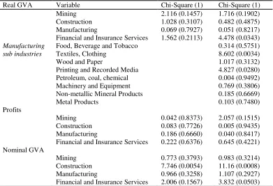
Table 4. Testing for valid over-identification restrictions
Real GVA Variable Chi-Square (1) Chi-Square (1) Mining 2.116 (0.1457) 1.716 (0.1902) Construction 1.028 (0.3107) 0.482 (0.4875) Manufacturing 0.069 (0.7927) 0.051 (0.8217) Financial and Insurance Services 1.562 (0.2113) 4.478 (0.0343) Manufacturing
sub industries
Food, Beverage and Tobacco 0.314 (0.5751)
Textiles, Clothing 8.602 (0.0034)
Wood and Paper 1.017 (0.3132)
Printing and Recorded Media 4.827 (0.0280) Petroleum, coal, chemical 0.004 (0.9492) Machinery and Equipment 0.769 (0.3806) Non-metallic Mineral Products 0.185 (0.6669)
Metal Products 0.103 (0.7480)
Profits
Mining 0.042 (0.8373) 2.057 (0.1515) Construction 0.083 (0.7726) 0.005 (0.9435) Manufacturing 0.186 (0.6660) 0.040 (0.8417) Financial and Insurance Services 0.222 (0.6376) 0.645 (0.4221) Nominal GVA
Mining 0.773 (0.3793) 0.983 (0.3214) Construction 7.746 (0.0054) 11.16 (0.0008) Manufacturing 0.966 (0.3258) 1.107 (0.2927) Financial and Insurance Services 2.006 (0.1567) 3.832 (0.0503)
The null hypothesis that the over identification restrictions are valid. Test statistics are reported, p-values are in parenthesis. Left column shows statistics for the baseline model, right shows the extended model.
Table 5.Testing for unit roots
Variable ADF KPSS Variable ADF KPSS
-1.523 2.744*** -4.652*** 0.356*
1.304 2.723*** -7.745*** 0.269
-0.184 1.977*** -4.709*** 0.273
-2.387 2.780*** -4.185*** 0.452*
-1.398 2.661*** -7.188*** 0.169
-0.079 2.663*** -5.167*** 0.067
-4.624*** 0.072
0.685 2.558*** ∆ -4.416*** 0.404*
-6.041*** 0.115
-0.230 2.255*** -5.634*** 0.116
) -0.475 1.951*** ) -5.436*** 0.195
) -1.516 1.031*** ) -5.819*** 0.133
) -1.904 1.373*** ) -5.252*** 0.057 The null hypothesis is that the variable has a unit root. ***, **, * denotes rejection of the null hypothesis
at the 1%, 5% and 10% level. ∆ denotes first difference. Lag length is 2. Only intercept included in the
[image:29.595.116.530.416.584.2]Figure 1.Disaggregated RBA index of commodity prices in United States dollars
Figure 2. Largest trading partners of Australia in terms of total trade value
0% 5% 10% 15% 20% 25%
1993 1995 1997 1999 2001 2003 2005 2007 2009 2011 2013
P
er
ce
nt
ag
e
of
A
us
tr
al
ia
's
T
ot
al
T
ra
de
V
al
ue
[image:30.595.117.540.309.524.2]
Figure 3. Response of industry variables to a 1% commodity price shock -0.4 -0.3 -0.2 -0.1 0 0.1
1 3 5 7 9 11 13 15 17 19
Quarters
Real GVA Mining
-0.2 -0.1 0 0.1 0.2 0.3
1 3 5 7 9 11 13 15 17 19
Quarters
Real GVA Manufacturing
-0.1 0 0.1 0.2 0.3 0.4 0.5 0.6 0.7
1 3 5 7 9 11 13 15 17 19
Quarters
Real GVA Construction
-0.3 -0.2 -0.1 0 0.1 0.2
1 3 5 7 9 11 13 15 17 19
Quarters
Real GVA Financial
0 1 2 3 4 5 6
1 3 5 7 9 11 13 15 17 19
Quarters Profits Mining -3 -2 -1 0 1 2
1 3 5 7 9 11 13 15 17 19
Quarters Profits Construction -10 -5 0 5 10 15
1 3 5 7 9 11 13 15 17 19
Quarters Profits Financial -2 -1 0 1 2
1 3 5 7 9 11 13 15 17 19
Quarters Profits Manufacturing -0.5 0 0.5 1 1.5 2
1 3 5 7 9 11 13 15 17 19
Quarters
Nominal GVA Mining
-0.3 -0.2 -0.1 0 0.1 0.2
1 3 5 7 9 11 13 15 17 19
Quarters
Nominal GVA Manufacturing
-0.2 0 0.2 0.4 0.6 0.8 1
1 3 5 7 9 11 13 15 17 19
Quarters
Nominal GVA Construction
-0.1 0 0.1 0.2 0.3 0.4
1 3 5 7 9 11 13 15 17 19
Quarters
Figure 4. Response of industry variables to a 1% bulk commodity price shock
Figure 5. Responses of manufacturing sub industry real GVA to a 1% bulk commodity price shock
-0.2 -0.1 0 0.1
1 3 5 7 9 11 13 15 17 19
Quarters Food, Beverage and Tobacco
Products
-0.3 -0.2 -0.1 0 0.1 0.2
1 3 5 7 9 11 13 15 17 19
Quarters Textiles, Clothing and Other
Manufacturing
-0.1 0 0.1
0.2 Petroleum, Coal, Chemical and
Rubber Products
0 0.1 0.2
0.3 Machinery and Equipment
0 0.1 0.2 0.3 0.4
1 3 5 7 9 11 13 15 17 19
Quarters
Non-Metallic Mineral Products
-0.1 0 0.1
[image:32.595.112.541.590.815.2]Figure 6. Response of industry variables to a 1% base metals shock -0.4 -0.3 -0.2 -0.1 0 0.1
1 3 5 7 9 11 13 15 17 19
Quarters
Real GVA Mining
-0.1 0 0.1 0.2 0.3
1 3 5 7 9 11 13 15 17 19 Quarters
Real GVA Manufacturing
-0.2 -0.1 0 0.1 0.2 0.3 0.4 0.5
1 3 5 7 9 11 13 15 17 19
Quarters
Real GVA Construction
-0.2 -0.1 0 0.1 0.2
1 3 5 7 9 11 13 15 17 19
Quarters
Real GVA Financial
-2.5 -2 -1.5 -1 -0.5 0 0.5 1 1.5 2
1 3 5 7 9 11 13 15 17 19
Quarters Profits Mining -1.5 -1 -0.5 0 0.5 1 1.5 2
1 3 5 7 9 11 13 15 17 19 Quarters Profits Manufacturing -2 -1.5 -1 -0.5 0 0.5 1 1.5 2
1 3 5 7 9 11 13 15 17 19
Quarters Profits Construction -10 -5 0 5 10 15 20
1 3 5 7 9 11 13 15 17 19
Quarters Profits Financial 0 0.1 0.2 0.3 0.4 0.5 0.6 0.7 0.8
1 3 5 7 9 11 13 15 17 19
Quarters
Nominal GVA Mining
0 0.1 0.2 0.3 0.4 0.5
1 3 5 7 9 11 13 15 17 19
Quarters
Nominal GVA Manufacturing
-0.1 0 0.1 0.2 0.3 0.4 0.5 0.6
1 3 5 7 9 11 13 15 17 19
Quarters
Nominal GVA Construction
-0.2 -0.1 0 0.1 0.2
1 3 5 7 9 11 13 15 17 19
Quarters
Figure 7. Response of industry variables to a 1% rural commodityprice shock -0.2 -0.1 0 0.1 0.2
1 3 5 7 9 11 13 15 17 19
Quarters
Real GVA Mining
-0.2 -0.1 0 0.1
1 3 5 7 9 11 13 15 17 19 Quarters
Real GVA Manufacturing
-0.2 -0.1 0 0.1 0.2 0.3
1 3 5 7 9 11 13 15 17 19
Quarters
Real GVA Construction
-0.1 0 0.1 0.2 0.3
1 3 5 7 9 11 13 15 17 19 Quarters
Real GVA Financial
-1 -0.5 0 0.5 1 1.5 2
1 3 5 7 9 11 13 15 17 19
Quarters Profits Mining -0.8 -0.6 -0.4 -0.2 0 0.2 0.4 0.6 0.8 1
1 3 5 7 9 11 13 15 17 19 Quarters Profits Manufacturing -2 -1.5 -1 -0.5 0 0.5 1
1 3 5 7 9 11 13 15 17 19
Quarters Profits Construction -8 -6 -4 -2 0 2 4 6 8 10
1 3 5 7 9 11 13 15 17 19
Quarters Profits Financial -0.2 -0.1 0 0.1
1 3 5 7 9 11 13 15 17 19 Quarters
Nominal GVA Manufacturing
-0.1 0 0.1 0.2 0.3 0.4 0.5 0.6 0.7
1 3 5 7 9 11 13 15 17 19
Quarters
Nominal GVA Construction
0 0.1 0.2 0.3
1 3 5 7 9 11 13 15 17 19
Quarters
Nominal GVA Financial -0.1 0 0.1 0.2 0.3 0.4 0.5 0.6 0.7 0.8
1 3 5 7 9 11 13 15 17 19 Quarters
Figure 9. Impulse responses of domestic variables to 1% innovations
Appendix A: Data description and sources
Variable Source Transformation
Gross domestic product in real US dollars (Datastream codes: EXXGDP$.C, USXGDP$.C, JPXGDP$.C, CHXGDP$.C, UKXGDP$.D)
Each countries’ series are seasonally adjusted using a moving average.
Consumer price index: all items
(Datastream codes: UKXCPI..F, USXCPI..E, CHXCPI..F, JPXCPI..F, EKXCPI..F)
Each countries’ series are seasonally adjusted using a moving average.
Interest rate: central bank policy rate
(Datastream codes: EKXRCB..R, CHXRCB..R, JPXRCB..R, UKXRCB..R, USXRCB..R)
,
Index of commodity prices, all items, bulk commodities, base metals and rural commodities in US dollars (RBA, Statistical Table G5)
Deflated by the US CPI for all Urban Consumers (FRED)
Seasonally adjusted chain volume measure of non-farm gross domestic product (ABS Cat No 5206.0, Table 6)
Seasonally adjusted chain volume measure of industry gross value added, (ABS Cat. No. 5206.0, Table 6)
Current price industry gross value added (ABS Cat. No. 5204.0, Table 5)
Data is converted from annual into quarterly data by using simple linear interpolation.
Seasonally adjusted, current price company profits before income tax in percentage change (ABS Cat. No. 5676.0, Table 10)
Outliers have been removed.
All groups consumer price index, 1989/90 = 100, excluding interest and tax changes of 1999—2000 (RBA Statistical Table G1)
Quarterly average of the target cash rate (RBA Statistical Table F1)
Converted from monthly to quarterly using a 3-month average.
Real trade-weighted index, March 1995=100 (RBA Statistical Table F15)
Appendix B: Test for model suitability
Sensitivity Analysis (Autocorrelation and heteroskedasticity tests)
The residual serial correlation LM test is used to test for first order autocorrelation. Of
the 38 models estimated, the null hypothesis of no first order serial correlation cannot be
rejected at the 10 per cent level for 36 of the models (nominal GVA of both mining and
professional services, in the baseline model exhibit first order serial correlation).
The residual heteroskedasticity LM test is also estimated for all 38 models, and in each
case the null hypothesis of no heteroskedasticity of the join combinations of all error