Representative scenario construction and preprocessing for robust combinatorial optimization problems

(will be inserted by the editor)

Representative Scenario Construction and Preprocessing

for Robust Combinatorial Optimization Problems

Marc Goerigk · Martin Hughes

Received: date / Accepted: date

Abstract In robust combinatorial optimization with discrete uncertainty, ap-proximation algorithms based on constructing a single scenario representing the whole uncertainty set are frequently used. One is the midpoint method, which uses the average case scenario. It is known to be an N-approximation, whereN is the number of scenarios.

In this paper, we present a linear program to construct a representative scenario for the uncertainty set, which gives an approximation guarantee that is at least as good as for previous methods. We further employ hyper heuristic techniques operating over a space of preprocessing and aggregation steps to evolve algorithms that construct alternative representative single scenarios for the uncertainty set.

In numerical experiments on the selection problem we demonstrate that our approaches can improve the approximation guarantee of the midpoint approach by more than 20%.

Keywords robust optimization·combinatorial optimization·approximation algorithms·scenario reduction·scenario preprocessing

1 Introduction

We consider combinatorial optimization problems of the general form

min

x x x∈Xcccxxx

Partially funded through EPSRC grants EP/L504804/1 and EP/M506369/1.

M. Goerigk and M. Hughes Department of Management Science Lancaster University

United Kingdom Tel.: +44-1524-595125

where ccc ≥000 is a cost vector, and X ⊆ {0,1}n _{is a set of feasible solutions.}

As real-world problems may suffer from uncertainty, robust counterparts to combinatorial problems have been considered in the literature, see [2, 9] for surveys on the topic. The resulting robust (or min-max) optimization problem is then of the form

min

x x

x∈Xmaxccc∈Ucccxxx (MinMax)

whereUcontains all possible cost vectorsccc1_{, . . . , ccc}N _{against we wish to protect.}

As robust combinatorial problems are usually NP-hard, approximation methods have been considered [1]. Two such heuristics stand out in the lit-erature, the midpoint and the element-wise worst-case algorithm, as they are easy to use and implement, and have been providing the best-known approxi-mation guarantee for a wide range of problems. While this guarantee has been improved for specific problems, they are still the best-known general methods (see [5]). Both algorithms are based on constructing a single scenario that rep-resents the whole uncertainty U. For the midpoint algorithm, we use ˆccc with ˆ

cj = 1/NPi∈[N]c

i

j for allj ∈[n]. For the element-wise worst-case algorithm,

we setcccby usingcj = maxi∈[N]cij. Let us denote byxxx(ccc) a minimizer for the

nominal problem with costsccc, and set ˆxxx:=xxx(ˆccc) (the midpoint solution) and

xxx:=xxx(ccc) (the element-wise worst-case solution). The following results can be found in [2].

Theorem 1 The midpoint solutionxxxˆ is an N-approximation for _MinMax.

Theorem 2 The element-wise worst-case solution xxxis an N-approximation for MinMax.

Frequently, problems with ”nice” structure (such as shortest path, spanning tree, selection, or assignment) have been considered in the literature, where it is possible to solve the nominal problem in polynomial time. In particular, this setting makes it possible to solve both of the above approaches in polynomial time by solving one specific scenario (i.e., findingxxx(ˆccc) orxxx(ccc)). This can then be used, e.g., as part of a branch and bound procedure for the (hard) robust problem.

The approximation guarantees from Theorems 1 and 2 are tight, as the following two examples for robust shortest path problems demonstrate (see also [2]).

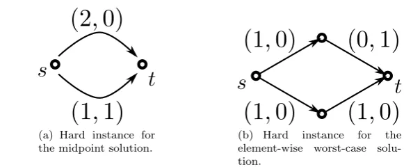
In Figure 1(a), the midpoint solution cannot distinguish between the upper edge and the lower edge. Hence, in this case, theN-approximation guarantee is tight with N = 2. In Figure 1(b), the element-wise worst-case solution cannot differentiate between the upper and the lower path. This instance is an example where theN-approximation guarantee is tight for this approach.

(a) Hard instance for the midpoint solution.

(b) Hard instance for the element-wise worst-case solu-tion.

Fig. 1 Example instances for robust shortest path with two scenarios.

edges are required. This demonstrates that the midpoint solution is not ann -approximation, whereas it is easy to show that this is the case for the element-wise worst-case approach.

Recently, data-driven robust optimization approaches have been investi-gated in the literature (see, e.g., [3, 8]). This paper has a similar research out-look by using the available data for better approximation guarantees, instead of ignoring structure that may be present. In a similar spirit, by analyzing the symmetry of an uncertainty set, [6] is able to derive improved approximation bounds for the related_{MinMax Regret} problem with compact uncertainty sets.

One general approach for the automated design of search heuristics is the use of hyper heuristics (see, e.g., [4, 10]). Hyper heuristics encompass search methods that operate on the space of search heuristics, constructing improved search approaches.

2 Scenario construction based on the midpoint approach

LetOP T be the optimal objective value of problemMinMax, and letxxx∗ be any optimal solution. Let some scenarioccc(not necessarily inU) be given. Then

U B(ccc) = max

i∈[N]

cccixxx(ccc)

is an upper bound onOP T. If it is possible to compute a lower bound from

ccc, we denote this asLB(ccc), and a bound on the ratio as

r(ccc)≥U B(ccc)/LB(ccc)

We call r(ccc) an a-priori bound, if it does not require the computation of

xxx(ccc) to find. Otherwise, we call it ana-posteriori bound. The reason for this distinction is that calculation ofxxxcan be costly, if the nominal problem is not solvable in polynomial time.

As an example, the midpoint method uses ˆccc:= _N1 P

i∈[N]ccc

i_{. It comes with}

an a-priori bound that isN, but by usingLB(ˆccc) = ˆcccxxx(ˆccc), we can calculate a stronger a-posteriori bound.

We now consider the problem of finding a better a-priori bound than N. To this end, note that Theorem 1 can be proven in the following way.

Proof (of Theorem 1)

U B(ˆccc) = max

i∈[N]

cccixxxˆ (i)

≤Nˆcccxxˆx≤Nˆcccxxx∗

(ii)

≤ Nmax

i∈[N]

cccixxx∗=N·OP T

u t

To mirror the steps of this proof, let us consider the following optimization problem:

min

t,ccc t (1)

s.t. max

i∈[N]ccc

i_{xxx(ccc)≤t·cccxxx(ccc) (2)}

cccxxx∗≤max

i∈[N]ccc

i_xxx∗ ₍₃₎

Lemma 1 Let (t, ccc)be a feasible solution to Problem (1–3). Then, xxx(ccc) is a

t-approximation for _MinMax.

Proof Analogous to the proof of Theorem 1: Constraint (2) ensures

Inequal-ity (i), while Constraint (3) ensures Inequality (ii). ut

Note that Problem (1–3) cannot be solved directly, as both the optimal solution

Lemma 2 Letccc fulfil X

j∈S

ci_j≤tX

j∈S

cj ∀i∈[N], S⊆[n] :|S|=k (4)

for some value of t, and constant k such that k ≤ P

j∈[n]xj for all x ∈ X. Then, (t, ccc)also fulfils (2).

Proof Let X = {j ∈ [n] : xj(ccc) = 1} and S ={S ⊆[n] : |S| = k, S ⊆ X}.

Then, the number of setsSin S containing a specific itemj∈X is the same for allj. Let`be this number. By summing (4) over allS∈ S, we find that

`X

j∈X

ci_j≤t`X

j∈X

cj ∀i∈[N]

and the claim follows. ut

Note that for constant k, it is possible in polynomial time to check if k ≤ P

j∈[n]xj for allx∈ X. Also, the setS contains polynomially many elements.

As an example, fork= 1, Constraint (4) becomes

ci_j ≤tcj ∀i∈[N], j∈[n]

and fork= 2, it becomes

ci_j+ci<sub>`</sub>≤t(cj+c`) ∀i∈[N], j, `∈[n], j6=`

In general, the constraints for some fixedkalso imply the constraints for any larger k. This means that the larger the value of k, the larger is the set of feasible solutions to our optimization problem, and the better approximation guarantees we can get.

Lemma 3 Letccc be inconv(U) =conv{ccc1_{, . . . , ccc}N_{}. Then,cccfulfils (3).}

Proof Letccc=P

i∈[N]λiccciwithPi∈[N]λi = 1 andλi≥0 for alli∈[N]. Then,

for anyxxx∈ X,

cccxxx= X

i∈[N]

λicccixxx≤

X

i∈[N]

λimax j∈[N]ccc

j_{xxx= max} j∈[N]ccc

j_xxx

u t

We now consider the following linear program:

maxt (5)

s.t.tX

j∈S

ci_j ≤X

j∈S

cj ∀i∈[N], S⊆[n] :|S|=k (6)

ccc= X

i∈[N]

X

i∈[N]

λi= 1 (8)

λi≥0 ∀i∈[N] (9)

Note that we replaced variabletin Problem (1–3) with 1/tto linearize terms.

Theorem 3 Let(t∗, ccc∗)be an optimal solution to Problem (5–9). Then,xxx(ccc∗)

is a1/t∗-approximation for MinMax, and1/t∗≤N.

Proof By Lemmas 2 and 3, (1/t∗, ccc∗) is feasible for Problem (1–3). Using

Lemma 1, we therefore find thatxxx(ccc∗) is a 1/t∗-approximation forMinMax. To see that 1/t∗ ≤ N, note that (1/N,cccˆ) is a feasible solution to

Prob-lem (5–9). ut

We note that if one uses the proof of Theorem 2 as a starting point, the same optimization problem can be derived.

Once a solution (t∗, ccc∗) has been computed, we have found an a-priori approximation guarantee. If we then compute xxx(ccc∗), we can derive a lower boundccc∗_xxx(ccc∗_{), asccc}∗_{∈conv(U), and an upper bound by calculating the}

objec-tive value ofxxx(ccc∗_{) for}

MinMax. This way, a stronger a-posteriori guarantee is found.

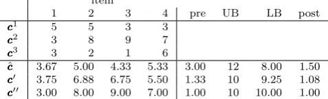
Example 1 We illustrate our approach using a small selection problem as an

example. Given four items, the task is to choose two of them that minimize the worst-case costs over three scenarios. The upper part of Table 1 shows the item costs in each scenario.

item

1 2 3 4 pre UB LB post

ccc1 _{5 5 3 3}

ccc2 _{3 8 9 7}

ccc3 _{3 2 1 6}

ˆ

ccc 3.67 5.00 4.33 5.33 3.00 12 8.00 1.50

ccc0 _{3.75 6.88 6.75 5.50 1.33 10 9.25 1.08}

ccc00 _{3.00 8.00 9.00 7.00 1.00 10 10.00 1.00}

Table 1 Example item costs, with midpoint scenario (ˆccc), our LP-based scenario withk= 1 (ccc0_{), and withk= 2 (ccc}00_).

The midpoint scenario (i.e., the average in each item) is shown in the row below (ˆccc). An optimal solution for this scenario is to pack items 1 and 3. This means that we have an a-priori approximation ratio of N = 3, and can calculate a lower bound LB(ˆccc) = ˆcccxxxˆ = 8 and an upper bound U B(ˆccc) = maxi∈[N]cccixxxˆ = 12. Combining lower and upper bound, we find the stronger a-posteriori bound of 1.50.

optimal solution is to take items 1 and 4. Accordingly, we find a lower bound of 9.25, an upper bound of 10, and an a-posteriori ratio of 1.08.

Finally, we also use our LP with k = 2 to find the scenarioccc00 and an a-priori guarantee of 1. This means that even before we have solved the problem, we already know that the resulting solution will be optimal. Indeed, we find that packing items 1 and 4 gives the optimal solution with objective value 10.

Note that we can also use the linear program (5–9) to strengthen the approximation guarantee of the midpoint scenario ˆcccwithout calculating ˆxxx, by only keepingtvariable.

We conclude this section by introducing an alternative approach to calcu-late a-posteriori bounds, which cannot be used for a-priori bounds. To this end, note that

max

c c

c∈conv(U)xminxx∈Xcccxxx≤minxxx∈Ximax∈[N]ccc

i_xxx

If the nominal problem can be written as a linear program, it can be dualized to find a compact formulation for the max-min problem. As both ˆccc and the optimal solution to problem (5–9) are inconv(U), this approach will result in a lower bound which will be at least as good as the lower bounds of the other two approaches. This may not result in a better ratio between upper and lower bound, however. We will test this approach in the experimental section.

3 Boundaries of scenario construction

Let us consider the more general optimization problem of constructing a sce-nario ccc∗_{, such that the resulting solution xxx(ccc}∗_{) has a good robust objective}

value. Formally, this amounts to

min

ccc∗_∈Ymax_ccc∈U cccxxx(ccc

∗_{) (}

ScenGen)

Note that (ScenGen) differs from (MinMax) by restricting the choice of solutionsxxxto only those which are optimal for a specific scenario. We write X0_{={xxx∈ X :∃ccc∈ Y s.t.cccxxx≤cccxxx}0 _∀xxx0_{∈ X }.}

For the set Y ⊆ Rn, different choices are possible. We discuss the three

natural approaches of usingY =_Rn_{, Y=U, orY=conv(U).}

In the first case of Y = _Rn_{, we get X}0 _{= X, i.e., we can construct any}

desired solution xxx(ccc) by setting cj to be low for elements where we want

xj(ccc) = 1, and by setting cj to be sufficiently high for elements where we

desire xj(ccc) = 0. This way, we find an optimal solution to (MinMax) by

solving (_ScenGen); at the same time, this setting does not appear tractable, so no advantage is reached.

The second case of Y = U is already discussed as a heuristic approach in [2], where an example is provided that the resulting solution does not give an approximation guarantee (i.e., can become arbitrarily bad).

to conv(U). We show that no such scenario can lead to a better than N -approximation algorithm. LetN+ 1 items be given, and exactly one of them needs to be chosen. There are N scenarios, where ci_j = N for i ∈ [N] if

i = j, and ci

N+1 = 1 +ε for some small ε > 0. All other values are zero. Letccc∗ ∈ conv(U), i.e., there is aλλλ ∈ [0,1]N _with P

i∈[N]λi = 1, such that

ccc∗ =P

i∈[N]λiccci. Leti∗ = arg mini∈[N]λi. Then,c∗i∗<= 1. Asc∗_N+1 = 1 +ε, an optimal solutionxxx(ccc∗) will not choose itemN+ 1, i.e., the optimal solution

xxx∗is not contained inX0_.

4 Evolving heuristics

We use the scenario construction approach from Section 2 as part of a hy-per heuristic, i.e., an optimization over the space of possible algorithms. Each algorithm consists of a sequence of preprocessing steps, where the set of sce-narios is modified, and an aggregation step, where the modified uncertainty set is reduced to a single scenario. The resulting one-scenario problem is then solved to optimality. Our aim is to find stronger upper bounds, at the cost of ignoring the approximation guarantee.

In the following, we first discuss possible aggregation and preprocessing steps, and then explain the genetic algorithm that searches the space of pos-sible heuristics.

4.1 Aggregation steps

Given a (modified) set of scenariosU ={ccc1, . . . , cccN}, the following six possible aggregation steps were considered:

1. AGG-EWC: the element-wise worst-case (see Section 1)

2. AGG-ARITH: the arithmetic mean, i.e., the midpoint approach (see Sec-tion 1)

3. AGG-MEDIAN: the median in each problem dimension 4. AGG-GEOM: the geometric mean in each problem dimension 5. AGG-HARMO: the harmonic mean in each problem dimension 6. AGG-LP: our scenario construction approach from Section 2

4.2 Preprocessing steps

Given a (modified) set of scenariosU ={ccc1, . . . , cccN}, the following eight possi-ble preprocessing steps were considered. Most of them require further param-eters, which are also listed below.

1. EMPTY: The uncertainty set is not modified.

3. MERGE(NORM,FLOAT): Repeat the following FLOAT·N many times: For each pair of scenariosi, j∈[N], calculate NORM(ccci−cccj). Choose the pair (i∗, j∗) for which this value is minimal, and replace these two scenarios withccc0= 0.5·(ccci∗+cccj∗).

4. NONDOM: Remove all dominated scenarios, i.e., removeccci _{if there exists}

ccck_6=ccci _{such thatc}k

j ≥cij for allj∈[n].

5. CONVEX: Remove all scenarios that lie in the convex hull of the other scenarios. To determine if this is the case, we solve a linear program for each scenario.

6. SCALE(FLOAT,AGG): Calculate a scenarioccc0through AGG, and setccci_←

FLOAT·ccc0+ (1−FLOAT)·ccci _{for all i ∈ [N]. Note that the number of}

scenarios is not reduced.

7. SAMPLE(FLOAT,INT): We sample a setX0 _{⊆ X with cardinality INT of}

random feasible solutions. For eachi∈[N], we then calculate the average costs avi = 1/|X0| ·Pxxx∈X0cccixxx. Remove the FLOAT·N scenarios with smallest costs avi.

8. KMEANS(FLOAT): Use a K-means heuristic to find (1−FLOAT)·N

clusters of scenarios. Replace each cluster through the average of scenarios belonging to this cluster.

The possible parameter values we considered are:

– NORM may be k · k1,k · k2,k · k22, or k · k∞ – DIR may be “smallest” or “largest”

– FLOAT my be any real in [0,0.3]

– INT may be any integer in [0,1000]

– AGG may be any aggregation type from Section 4.1

4.3 Genetic algorithm

The preprocessing and aggregation steps from Sections 4.1 and 4.2 are com-bined to form heuristic algorithms for problem _MinMax. To this end, we fix that each algorithm does exactly six preprocessing steps, and then one ag-gregation step. This reduces the number of scenarios to one. The resulting nominal problem is then solved to optimality.

A set of such algorithms (individuals) forms a population, which is iter-atively improved using a simple linear genetic programming approach based on a genetic algorithm. We evaluate each individual on a set of problem in-stances, and record the average of the ratios between resulting objective value and optimal objective value, as well as the computation time. Both values are used to determine the fitness of an individual in a bicriteria way as described in [7], that is, by determining a Pareto rank and a crowdedness value. The for-mer promotes individuals that are less dominated, while the latter promotes a population that is evenly spread.

This way, we include the midpoint method and the element-wise worst-case approach. Additionally, we sample random algorithms until a fixed population size is reached.

To determine a subsequent population, we double the population size by choosing random pairs of individuals, crossing them, and mutating them. To cross two individuals, we randomly choose preprocessing steps and the ag-gregation step from each with equal probability. To mutate an individual, we randomly change preprocessing steps, their parameters, and the aggregation step with low probability. We then halve the population back to the original size using 2-tournaments.

We iterate this process until an iteration limit is reached. The result is an improved set of algorithms that represents a trade-off between computation time and objective value performance.

5 Experiments

We conduct two sets of experiments. In the first set, we focus on the quality of bounds generated through our scenario generation approach. In the second set, we evolve heuristics as described in Section 4. For all experiments we used a computer with a 16-core Intel Xeon E5-2670 processor, running at 2.60 GHz with 20MB cache, and Ubuntu 12.04. We used CPLEX v.12.6 to solve all problem formulations, and a C++ library by John Burkardt 1 for K-means computations.

5.1 Experiment 1: Bounds

5.1.1 Setting

To test the quality of our LP-based scenario construction approach, we con-sider instances of the selection problem (see, e.g., [9]). Here,X ={xxx∈ {0,1}n_:

P

j∈[n]xj =p} for some integer parameter p. We generate item costscij by

sampling uniformly i.i.d. from {0,1, . . . ,100}. We use N ∈ {2,5,10,50,100} for smaller instances with n = 10, p= 3 and larger instances with n = 30,

p= 9. For each parameter combination, we generate 1000 instances and aver-age results.

5.1.2 Results

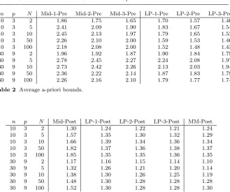
Table 2 shows the a-priori bounds for the midpoint approach when using our linear program (5–9) for evaluation with k = 1, k = 2 and k = 3 (Mid-1-Pre, Mid-2-(Mid-1-Pre, and Mid-3-(Mid-1-Pre, respectively). We compare this to the a-priori bounds that are found when also optimizing over the scenario ccc for k = 1,

k = 2 and k = 3 (LP-1-Pre, LP-2-Pre, and LP-3-Pre, respectively). Note

1

n p N Mid-1-Pre Mid-2-Pre Mid-3-Pre LP-1-Pre LP-2-Pre LP-3-Pre

10 3 2 1.86 1.75 1.65 1.70 1.57 1.46

10 3 5 2.41 2.09 1.90 1.83 1.67 1.54

10 3 10 2.45 2.13 1.97 1.79 1.65 1.53

10 3 50 2.26 2.10 2.00 1.59 1.53 1.46

10 3 100 2.18 2.08 2.00 1.52 1.48 1.43

30 9 2 1.96 1.92 1.87 1.90 1.84 1.79

30 9 5 2.78 2.45 2.27 2.24 2.08 1.97

30 9 10 2.73 2.42 2.26 2.13 2.03 1.94

30 9 50 2.36 2.22 2.14 1.87 1.83 1.79

30 9 100 2.26 2.16 2.10 1.79 1.77 1.74

Table 2 Average a-priori bounds.

n p N Mid-Post LP-1-Post LP-2-Post LP-3-Post MM-Post

10 3 2 1.30 1.24 1.22 1.21 1.24

10 3 5 1.57 1.35 1.30 1.32 1.29

10 3 10 1.66 1.39 1.34 1.36 1.34

10 3 50 1.82 1.37 1.36 1.38 1.37

10 3 100 1.85 1.35 1.35 1.36 1.35

30 9 2 1.17 1.16 1.15 1.14 1.10

30 9 5 1.32 1.26 1.21 1.20 1.14

30 9 10 1.38 1.30 1.26 1.25 1.19

30 9 50 1.48 1.30 1.28 1.28 1.28

30 9 100 1.52 1.30 1.28 1.28 1.30

Table 3 Average a-posteriori bounds.

that overall, all guarantees are considerably smaller thanN. Furthermore, our approach is able to improve the bound of the midpoint algorithm. On average, the guarantee that the midpoint approach gives is more than 20% larger than our guarantee.

We contrast the a-priori bounds with a-posteriori bounds in Table 3, i.e., we calculate the solutionsxxx(ccc) for the respective scenarioscccand the resulting ratio of upper and lower bound. On average, the bound provided by the mid-point solution is around 17% larger than the bound provided by our approach with k = 2 or k = 3. The max-min approach (denoted by MM) performs slightly better than our approach (Mid-Post is on average 19% larger than MM-Post), but this comes without an a-priori guarantee, at the cost of higher computational effort, and it is not always possible to compute as explained in Section 2.

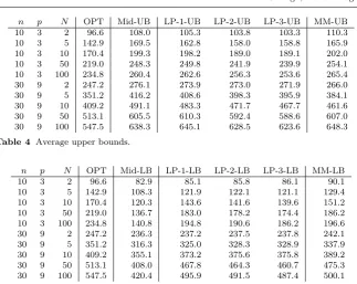
n p N OPT Mid-UB LP-1-UB LP-2-UB LP-3-UB MM-UB 10 3 2 96.6 108.0 105.3 103.8 103.3 110.3 10 3 5 142.9 169.5 162.8 158.0 158.8 165.9 10 3 10 170.4 199.3 198.2 189.0 189.1 202.0 10 3 50 219.0 248.3 249.8 241.9 239.9 254.1 10 3 100 234.8 260.4 262.6 256.3 253.6 265.4 30 9 2 247.2 276.1 273.9 273.0 271.9 266.0 30 9 5 351.2 416.2 408.6 398.3 395.9 384.1 30 9 10 409.2 491.1 483.3 471.7 467.7 461.6 30 9 50 513.1 605.5 610.3 592.4 588.6 607.0 30 9 100 547.5 638.3 645.1 628.5 623.6 648.3

Table 4 Average upper bounds.

n p N OPT Mid-LB LP-1-LB LP-2-LB LP-3-LB MM-LB 10 3 2 96.6 82.9 85.1 85.8 86.1 90.1 10 3 5 142.9 108.3 121.9 122.1 121.1 129.4 10 3 10 170.4 120.3 143.6 141.6 139.6 151.2 10 3 50 219.0 136.7 183.0 178.2 174.4 186.2 10 3 100 234.8 140.8 194.8 190.6 186.2 196.6 30 9 2 247.2 236.3 237.2 237.5 237.8 242.1 30 9 5 351.2 316.3 325.0 328.3 328.9 337.9 30 9 10 409.2 355.1 373.2 375.6 375.8 389.2 30 9 50 513.1 408.0 467.8 464.3 460.7 475.3 30 9 100 547.5 420.4 495.9 491.5 487.4 500.1

Table 5 Average lower bounds.

5.2 Experiment 2: Evolution

5.2.1 Setting

We generated 750 instances to train our genetic algorithm, and another set of 750 instances in the same way to evaluate our results. Each set consists of 250 instances of three types. Uniform instances, where item costs are generated uniformly i.i.d. in{1, . . . ,100}. Correlated instances, where for each item j, a nominal value ˆcj is chosen uniformly i.i.d. in {1, . . . ,100}. Scenarios are then

generated by sampling values from [0.7·ˆcj,1.3·cˆj]. And finally, instances where

for each item, exactly three distinct values chosen from {1, . . . ,100} can be attained. The smallest and highest values are each chosen with probability 10%, and the middle value with probability 80%.

We letnrun from 10 to 50, andKfrom 10 to 100 in steps of 10. We always setp= 0.25n. Each setting is repeated 5 times (this makes 5·10·5·3 = 750 instances). All problems were solved to find their respective optimal objective values.

Our genetic algorithm was run using a population of 30 individuals over 1,200 generations. As we inject possibly bad solutions after each iteration, the following evaluation only considers the 20 best individuals out of the available 30.

for the midpoint method without preprocessing, so that it remains part of the population over all iterations.

5.2.2 Results

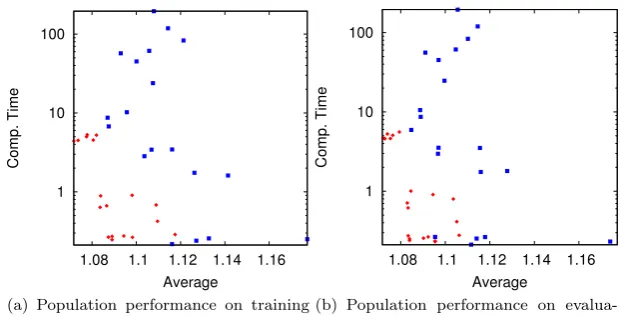
We summarize our results in Figure 2. In Figure 2(a), we show average ob-jective value ratios and total computation times on the (in-sample) training instances, using blue squares for the starting population, and red diamonds for the final population. The same is done in Figure 2(b) for the (out-sample) evaluation instances.

1 10 100

1.08 1.1 1.12 1.14 1.16

Comp. Time

Average

(a) Population performance on training set.

1 10 100

1.08 1.1 1.12 1.14 1.16

Comp. Time

Average

(b) Population performance on evalua-tion set.

Fig. 2 Experimental results for the evolution approach. Starting population as blue squares, and final population in red diamonds.

In Figure 2(b) one can observe a distinct clustering of the final population into two sets: Individuals with higher computation times but better objective values on the left, and individuals with better computation times but worse objective values bottom right from the first group. All six individuals from the first group use AGG-LP for the aggregation step, whereas the fourteen individuals from the second group use AGG-ARITH (10 times), AGG-EWC (twice), or AGG-MEDIAN (twice).

The best average objective value ratio with 1.0717 in-sample and 1.0729 out-sample has been reached by the following algorithm:

1. SCALE(0.22, AGG-ARITH) 2. SAMPLE(0.18, 21)

3. SCALE(0.17, AGG-ARITH) 4. SCALE(0.25, AGG-EWC)

This algorithm’s computation time in-sample is 4.40 seconds, and 4.60 seconds out-sample. As a representative of the group of faster algorithms not based on LP-AGG, we show the following individual (omitting empty slots):

1. SCALE(0.29, AGG-EWC) 2. SCALE(0.16, AGG-EWC) 3. AGG-ARITH

This methods reaches an in-sample ratio of 1.0874 (1.0834 out-sample) and takes 0.27 seconds both in-sample and out-sample. Note that both methods make use of multiple AGG parameters. The first method uses AGG-ARITH and AGG-EWC for scaling, and LP-AGG for the aggregation step. The sec-ond method uses a scaling towards EWC before aggregating with AGG-ARITH. In fact, all individuals of the final population (except the midpoint method) combine at least two aggregation techniques. Intuitively, this is a reasonable approach to ensure a robust performance, as focussing on a single aggregation technique may work well in some instances, but worse on others. By averaging multiple techniques, we achieve a better performance on average. The final population consists of 20 individuals, with five preprocessing slots each. Table 6 shows the frequency of preprocessing methods within these 100 available slots. MERGE and CONVEX were both not used at all.

EMPTY SCALE OUTLIER SAMPLE NONDOM KMEANS

44 32 13 7 2 2

Table 6 Frequency of preprocessing methods.

We can conclude that by using preprocessing on the scenario data it is pos-sible to achieve improved algorithms, which take only slightly longer to run, but produce better solutions. However, the potential of this approach is limited by the previous aggregation techniques. Using our LP-based approach, objec-tive values become significantly better, but at a price of higher computation times.

6 Conclusion

Most robust combinatorial optimization problems are hard, which has lead to the development of general approximation algorithms. The two best-known such approaches are the midpoint method and the element-wise worst-case approach. Both rely on creating a single scenario that is representative for the whole uncertainty set. By reconsidering the respective proofs that both are

N-approximation algorithms, we find an optimization problem to construct a representative scenario that results in an approximation which is at least as good as for the previous two scenarios.

that is about 20% larger than ours, while we only need to solve a simple linear program to construct the representative scenario. The improved a-priori guarantee is also reflected in an improved a-posteriori guarantee, with our approach providing both better upper and lower bounds than before. This smaller gap could potentially be used within branch-and-bound algorithms for a more efficient search for an optimal solution.

Additionally we used a hyper heuristic approach to develop algorithms to construct alternative single scenarios that best represent the whole uncertainty set in the subsequent solution of the resulting one-scenario robust combinato-rial problems.

References

1. Aissi, H., Bazgan, C., Vanderpooten, D.: Approximation of min–max and min–max regret versions of some combinatorial optimization problems. European Journal of Operational Research179(2), 281 – 290 (2007)

2. Aissi, H., Bazgan, C., Vanderpooten, D.: Min–max and min–max regret versions of com-binatorial optimization problems: A survey. European Journal of Operational Research

197(2), 427 – 438 (2009)

3. Bertsimas, D., Gupta, V., Kallus, N.: Data-driven robust optimization. Mathematical Programming167(2), 235–292 (2018)

4. Burke, E.K., Gendreau, M., Hyde, M., Kendall, G., Ochoa, G., ¨Ozcan, E., Qu, R.: Hyper-heuristics: a survey of the state of the art. Journal of the Operational Research Society64(12), 1695–1724 (2013)

5. Chassein, A., Goerigk, M.: On scenario aggregation to approximate robust optimization problems. Optimization Letters (2017). Available online, to appear.

6. Conde, E.: On a constant factor approximation for minmax regret problems using a symmetry point scenario. European Journal of Operational Research219(2), 452–457 (2012)

7. Deb, K., Pratap, A., Agarwal, S., Meyarivan, T.: A fast and elitist multiobjective ge-netic algorithm: Nsga-ii. IEEE transactions on evolutionary computation6(2), 182–197 (2002)

8. Dokka, T., Goerigk, M.: An Experimental Comparison of Uncertainty Sets for Ro-bust Shortest Path Problems. In: G. D’Angelo, T. Dollevoet (eds.) 17th Workshop on Algorithmic Approaches for Transportation Modelling, Optimization, and Systems (ATMOS 2017),OpenAccess Series in Informatics (OASIcs), vol. 59, pp. 16:1–16:13. Schloss Dagstuhl–Leibniz-Zentrum fuer Informatik, Dagstuhl, Germany (2017) 9. Kasperski, A., Zieli´nski, P.: Robust discrete optimization under discrete and interval

uncertainty: A survey. In: Robustness Analysis in Decision Aiding, Optimization, and Analytics, pp. 113–143. Springer (2016)