Optimized Face Recognition Technique based on PCA and RBF Neural Network

Optimized Face Recognition Technique based on

PCA and RBF Neural Network

Deepti Ahlawat

BPSMV Khanpur Kalan

Sonipat, Haryana

India

Vijay Nehra,

PhD

BPSMV Khanpur Kalan

Sonipat, Haryana

India

ABSTRACT

In the field of machine recognition and computer vision, face recognition using optimized Radial Basis Function (RBF) Network is a very efficient solution for the researchers working in this field. In face recognition, the main challenge is to obtain high recognition efficiency. In the present work, principal component method is used for feature extraction and feature reduction. The eigenvalues obtained are passed to the Radial Basis Function Network for classification. In this study, particle swarm optimization technique is used to optimize the centre and the width of the Radial Basis Function Network. The work is tested on three datasets: AT & T, Yale and CMU PIE. The results obtained show that the efficiency of the investigated work, in terms of recognition rate and the training time is better than existing neural Network based in Back Propagation.

Keywords

PCA, Radial Basis Function, Particle Swarm Optimization, face recognition

1. INTRODUCTION

In recent years, a lot of work has been done in the field of face recognition, pattern recognition etc. but still, in real time applications difficulties are faced by computer based systems due to noisy data, high dimensionality, facial appearance, orientation and changes in environmental conditions etc. These difficulties faced will affect the performance, accuracy and computational parameters of a classification technique. The aim of a classification problem is mapping of input to output class. The performance of an algorithm for the classificatory problems is measured by the number of inputs to which the algorithm could correctly determine the output class. The boundaries separating the various classes from each other in the feature space are called as the decision boundaries. Algorithms try to construct effective decision boundaries for classification purpose. The task is easy if the inter-class separation is high and intra-class separation is low. The problem is usually caused by data lying near the decision boundary which is usually difficult to classify. A number of classification algorithms have been proposed by a number of researchers for face recognition to improve the accuracy of the system and enhance the computational cost of the face recognition system.

A face recognition system includes two stages: 1) Firstly, detecting the location of face, which is a complicated task because of unknown position, scaling and orientation of face in any image and extracting features from the localized image. 2) Second stage involves the derived feature vectors for classification of the facial image [1]. Classifier play a crucial role in a recognition system, it should have faster speed and high accuracy.

PCA is a useful statistical technique which is given by Turk and Pentland, 1991 in [2], it is a way of extracts important features from the given database, and express the vectors in such a way as to highlight their similarities and differences. Since these vectors are hard to be found in data of high dimension. PCA reduces the data to low dimensional by calculating eigenvectors and eigenvalues of the covariance matrix of the train data and then carry on only largest eigenvectors corresponding to k largest eigenvalues. The test data is projected on these eigenvectors to reduce its dimensions. These features are then used for classification of the dataset.

Neural networks have been employed and compared to conventional classifiers for a number of classification problems. The results have shown that the accuracy of the neural network approaches equivalent to, or slightly better than, other methods. Also, due to the simplicity, generality and good learning ability of the neural networks, these types of classifiers are found to be more efficient [3].

Radial Basis Function (RBF) [4] neural networks have found to be very attractive for many engineering problem because: (1) they are universal approximators, (2) they have a very compact topology and (3) their learning speed is very fast because of their locally tuned neurons [1,5]. An important property of RBF neural networks is that they form a unifying link between many different research fields such as function approximation, regularization, noisy interpolation and pattern recognition. Therefore RBF neural networks serve as an excellent candidate for pattern applications and attempts have been carried out to make the learning process in this type of classification faster than normally required for the multilayer feed forward neural networks [6].

In the present work, optimized RBF neural network classifier is used for face recognition and for the first stage of face recognition Kernel-PCA (KPCA) is used for feature extraction which generates the features vectors to produce the high recognition accuracy.

2. PCA-RBF NEURAL NETWORK FOR

CLASSIFICATION

2.1 PCA approach for Feature Extraction

Principal Component Analysis [2] is a very powerful technique for feature extraction. The basic approach of PCA is to calculate the eigenvectors or principal components of the covariance matrix of the training data, and approximate it by a linear combination of the leading eigenvectors. To compute principal components consider a random vector 𝑋 = {𝑥1, 𝑥2, 𝑥3, 𝑥4… … … 𝑥𝑛} with observations 𝑥𝑖∈ ℝ𝑑. The mean 𝜇 is calculated by using equation (1)

𝜇 =1

𝑛 𝑥𝑖

𝑛

The covariance matrix S for the training database is computed using equation (2)

𝑆 =1

𝑛 (𝑥𝑖−

𝑛

𝑖=1 𝜇)(𝑥𝑖− 𝜇)𝑇 (2) The eigenvalues 𝜆 and eigenvectors 𝑣 of covariance matrix S is given by equation (3)

𝑆𝑣 = 𝜆𝑣 (3) The principal components are the largest eigenvectors corresponding to largest eigenvalues and small eigenvectors represent the noise. Hence 𝑘 principal components of the observed vector are chosen for describing the dataset which makes transformation matrix 𝑊 = (𝑣1, 𝑣2, 𝑣3, 𝑣4… … … 𝑣𝑘) is given by equation (4)

𝑦 = 𝑊𝑇_{(𝑥 − 𝜇) (4)} Following the above equations, PCA is used to extract the features which reduce the dimensions of the face database. In other words, the input face vector in 𝑛- dimensional space is reduced to a feature vector of 𝑘- dimensional subspace [2]. Hence dimensions of the reduced vector 𝑘 is much less than the dimension of input vector 𝑛. The calculated features are used to train the RBF neural network classifer.

2.2 Radial Basis Function

Radial Basis Function Networks (RBFN) are type of ANN that have one input layer, one hidden layer and one output layer. Its architecture is very similar to that of traditional three-layer feed forward neural network. Radial basis function networks have a number of applications, including function approximation, time series prediction, classification, and system control. These networks were first formulated in year 1988 by Broomhead and Lowe [7], both researchers at the Royal Signals and Radar Establishment.

[image:2.595.322.528.76.247.2]

The input layer of this network is a set of n units, which accept the elements of an n dimensional input feature vector. The input units are fully connected to the hidden layer with r hidden units. Connections between the input and hidden layers have unit weights and, as a result, do not have to be trained. The goal of the hidden layer is to cluster the data and reduce its dimensionality. In this structure hidden layer is named RBF units. The RBF units are also fully connected to the output layer. The output layer supplies the response of neural network to the activation pattern applied to the input layer. The transformation from the input space to the RBF-unit space is nonlinear (nonlinear activation function), whereas the transformation from the RBF-unit space to the output space is linear (linear activation function) [8]. The structure of RBF neural network is shown in figure 1. The input layer of this network is a set of 𝑛 units,which accept the elements of an 𝑛 -dimensional input feature vector, 𝑛 elements of the input vector x are input to the l hidden functions, the output of the hidden function, which is multiplied by the weighting factor w(i, j) , is input to the output layer of the network yj(x).

Fig. 1: Architecture of Radial Basis function Neural Network [9]

For each RBF unit , 𝑘, 𝑘 = 1,2,3 … … . , 𝑙, the centre is selected as the mean value of the sample patterns belong to class 𝑘, is calculated using equation (5)

𝜇𝑘= 1

𝑁𝑘 𝑥𝑘

𝑖_{, 𝑘 = 1,2,3, … . . , 𝑚} 𝑁𝑘

𝑖=1 (5) Where 𝑥_𝑘𝑖 _{is the eigenvector of the 𝑖 𝑡𝑕 image in the class 𝑘,} and 𝑁𝑘 is the total number of trained images in class 𝑘. Since the RBF neural network is a class of neural networks, the activation function of the hidden units is determined by the distance between the input vector and a prototype vector. Typically the activation function of the RBF units(hidden layer unit) is chosen as a Gaussian function with mean vector 𝜇𝑖 and variance vector 𝜎𝑖. The activation function is given by equation (6)

𝑕𝑖 𝑥 = 𝑒𝑥𝑝 − 𝑥−𝜇𝑖 2

𝜎𝑖 ,𝑖 = 1,2,3 … . . , 𝑙

(6)

Where . indicates the euclidean norm on the input space. Note that 𝑥 is an 𝑛- dimensional input feature vector, 𝜇𝑖 is an 𝑛- dimensional vector called centre of hidden layer, 𝜎𝑖 is the with if 𝑖 𝑡𝑕 RBF unit and 𝑙 is the number of hidden layer units [4,10]. The response of j 𝑡𝑕 output unit for input 𝑥 is given by equation (7)

𝑦𝑗 𝑥 = 𝑙 𝑕𝑖 𝑥 𝑤(𝑖, 𝑗)

𝑖=1 (7)

Where 𝑤(𝑖, 𝑗) is the connection weight of the 𝑖 𝑡𝑕 RBF unit to the j 𝑡𝑕 output node.

Hence, RBF network has a number of advantages which includes their generalization ability, tolerance to noise input and online learning ability [11]. These networks require very less training time as the weights are decided just by seeing the inputs. In the present investigation, the weights of Radial Basis function are optimized using Particle Swarm optimization algorithm. The detail of the optimization algorithm is given in the succeeding section.

3 OPTIMIZATION PARAMETERS OF

RBF NEURAL NETWORK

network as its internal learnable parameter s which are used in computing the output values and are learned and updated in the direction of optimal solution i.e minimizing the Loss by the network’s training process and also play a major role in the training process of the Neural Network Model. In literature, since decades a number of optimization algorithms have been proposed.

In the present investigation, the parameters of radial basis function are optimized using particle swarm optimization (PSO) algorithm. The PSO algorithm is discussed in brief:

3.1 Particle Swarm Optimization (PSO)

Algorithm

The Particle Swarm Optimization (PSO) [12] is a global optimization evolutionary approach, and provide a solution very close to the global solution. The optimization technique is inspired by the natural phenomenon of swarm movement i.e., birds flock in the sky, or fish schooling. If one of the particles discovers a good path to food the rest of the swarm will be able to follow instantly even if they are far away in the swarm. To describe the natural process used in this algorithm more technically the following steps are followed:

 The swarm is a population of particles which is randomly generated initially.

 Each particle represents a potential solution and has a

position represented by a position vector 𝑥𝑖= 𝑥𝑖1, 𝑥𝑖2, 𝑥𝑖3, … …. A swarm of particles moves

through the problem space, with the moving velocity of

each particle represented by a velocity vector 𝑣𝑖= 𝑣𝑖1, 𝑣𝑖2, 𝑣𝑖3, … ...

 Each group (or swarm) member do have its own position as well as velocity in a direction, called local best position, 𝑝𝑜𝑠𝑖(𝑡) pos t and local best velocity, 𝑣𝑙𝑜𝑐𝑎𝑙𝑖(𝑡), given by (8).

𝑣𝑙𝑜𝑐𝑎𝑙𝑖 𝑡 + 1 = 𝑐1𝑟1 𝑙𝑏𝑒𝑠𝑡𝑝 𝑡 − 𝑝𝑜𝑠𝑖(𝑡) (8)

 Group velocity, 𝑣𝑠𝑤𝑎𝑟𝑚𝑖(𝑡), can be calculated using (9), where, 𝑔𝑏𝑒𝑠𝑡𝑝(𝑡), denotes group best position 𝑣𝑠𝑤𝑎𝑟𝑚𝑖 𝑡 + 1 = 𝑐2𝑟2 𝑔𝑏𝑒𝑠𝑡𝑝 𝑡 − 𝑝𝑜𝑠𝑖(𝑡) (9)

 Best position amongst all local positions is treated as a global best position.

 The movement of the swarm is decided by the global best position and global best velocity.

Net velocity of the group can be calculated by (10) that adds an inertia coefficient 𝐼𝑐𝑖(𝑡) with it.

𝑣𝑒𝑙𝑖 𝑡 + 1 = 𝐼𝑐𝑖 𝑡 × 𝑣𝑙𝑜𝑐𝑎𝑙𝑖 𝑡 + 1 + 𝑣𝑠𝑤𝑎𝑟𝑚𝑖(𝑡 +

1)

(10) This inertia coefficient heads the direction of a particle (group member) in the direction of the optimal solution. Value of this parameter is given and updated as given in equation (11)

𝐼𝑐 = 𝐼𝑐𝑚𝑎𝑥 −𝐼𝑐𝑚𝑎𝑥−𝐼𝑐𝑚𝑖𝑛

𝑖𝑡𝑟𝑚𝑎𝑥 × 𝑖𝑡𝑟𝑘

(11)

Based on the group velocity, the position of i th member can be modified by equation (12)

𝑝𝑜𝑠𝑖 𝑡 + 1 = 𝑝𝑜𝑠𝑖 𝑡 + 𝑣𝑒𝑙𝑖(𝑡 + 1) (12)

PSO like other evolutionary algorithms needs a fitness function to be guided to a desired point. For this proposed method the fitness function will be designed considering the network accuracy and complexity. For the accuracy the RBF network in this article the mean squared network (MSE) is used. For this purpose the network with the architecture obtained from the particles in the swarm and the weights computed analytically is fed with the training dataset, the corresponding outputs are collected and compared with the desired outputs. The complexity of the network can be tracked by considering the number of the hidden units. The lower the number of hidden units is, the more desirable the fitness will be. Therefore the fitness function is given by equation (13):

𝑓𝑖𝑡𝑛𝑒𝑠𝑠 = _𝑁1 𝑁𝑖=1 𝑡𝑖− 𝑜𝑖 2+ 𝑘_{𝑀𝑎𝑥𝐻𝑖𝑑𝑑𝑒𝑛}𝑆𝑖𝑧𝑒𝐻𝑖𝑑𝑑𝑒𝑛 (13)

Where 𝑁 is the number of training patterns, 𝑘 is a balancing factor, 𝑡𝑖, 𝑜𝑖 are the desired output and actual network output respectively.

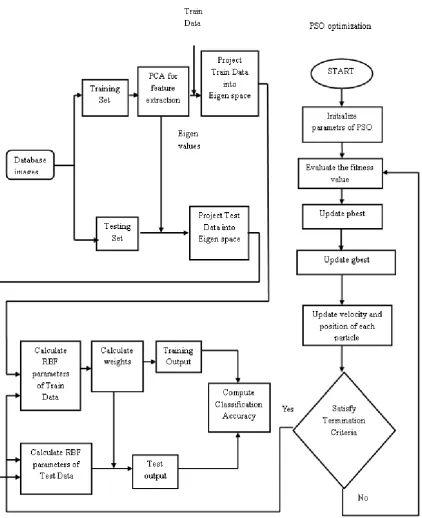
The pictorial representation of the optimization of parameters of RBF is illustrated in Figure 2.

4 EXPERIMENTAL RESULTS AND

DISCUSSION

4.1 Description of Dataset

In the present work, 3 datasets A T & T face database, CMU PIE dataset and Yale face database are considered to check the accuracy of the optimized PCA-RBF neural network. The description of each database is discussed below:

A. AT & T Database

To evaluate the efficiency of an algorithm AT & T dataset is the most popular dataset for the research purpose[13]. The database contains images of 40 individuals, where each individual consist of 10 images which are in .pgm format. AT &T dataset has a total of 400 images which includes facial expressions smiling faces and neutral faces, open and close eyes and facial details with and without glasses. Variable number of face images are used for training and experiments are conducted on rest of the images to calculate the classification accuracy of the proposed algorithm.

B. CMU PIE database

[image:4.595.106.529.72.591.2]

Fig 2: Flowchart of Optimized PCA-RBF Neural Network Classifier (Source: Own creation)

C. Yale Dataset

Yale face database consists of images of 15 individuals with the total of 165 gray scale images in .giff format [15]. All images are manually cropped to include only internal structures. The size of original image is 320 × 243 pixels. The main challenges in Yale face database are facial expressions (sad, sleepy, normal, happy, surprised, and wink), occlusion (with or without glasses) and misalignment along with illumination variations. For the experiment purpose neutral face are used for training and rest of the image for testing purpose.

4.2 Results and Discussion

The section presents the outcomes of the optimized PCA-RBF neural network in terms of accuracy and training time

[image:5.595.322.553.72.178.2]

neurons are set in the hidden layer. For the different number of training samples, we compute the training time for both the techniques PCA with neural network using Back Propagation algorithm and the proposed approach PCA using optimized RBF neural network with gradient descent activation function. From the results it can be analyzed that as the number of training samples are increased from 50 to 200 and also, testing sample are increased from 80 to 160 respectively the training time or the learning speed is raised from 32.11 to 60.1 seconds the maximum accuracy achieved is 95.1% with PCA and neural network using Back propogation. For the proposed technique as the training samples are increased from 50 to 200 and respective test samples from 80 to 160 the training time is increased from 27.4 to 54.32 sec with the maximum accuracy of 97.23%. Hence if we compare the two techniques for AT & T dataset, the proposed technique has better accuracy of 97.23% with the reduced training time.

Table 1: Comparison of training time (in seconds) and recognition accuracy of AT & T Database Techniq ue used Traini ng Sampl es Test Sampl es Neuro ns in hidden layer Traini ng time (in second s) Accura cy in %

PCA +Neural Network using BP

50 80 110 32.11 87.3

100 100 112 43.65 90.4

150 12 114 49.2 92.8

175 140 116 55.76 94.4

200 160 120 60.1 95.1

PCA+ Optimiz ed RBF neural Network

50 80 110 27.4 88.1

100 100 112 35.62 93.4

150 12 114 39.20 94.75

175 140 116 48.47 96.4

[image:5.595.318.549.230.459.2]

200 160 120 54.32 97.23

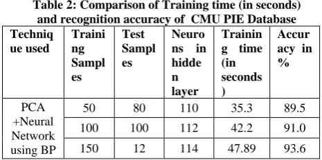
Table 2 presents the training time and accuracy of CMU PIE database with varying number of training images. For the BP classifier, as the number of training image samples are increased along with the test samples, the number of neurons in the hidden layer are also increased accordingly. For 200 training samples the number of neurons calculated are 120 with the training time of 57.24 and the recognition accuracy of 96.1%. Similarly, for optimized RBF classifier for 120 neurons in hidden layer, and 200 training samples the training time is 50.4 seconds and recognition accuracy is 98.63%. The proposed technique has a recognition rate of 2.53% more than the BP classifier.

Table 2: Comparison of Training time (in seconds) and recognition accuracy of CMU PIE Database Techniq ue used Traini ng Sampl es Test Sampl es Neuro ns in hidde n layer

Trainin g time (in seconds )

Accur acy in %

PCA +Neural Network using BP

50 80 110 35.3 89.5

100 100 112 42.2 91.0

150 12 114 47.89 93.6

175 140 116 53.11 94.9 200 160 120 57.24 96.1

PCA+ Optimiz ed RBF neural Network

50 80 110 24.89 89.9

100 100 112 29.311 93.88

150 12 114 37.20 95.0

175 140 116 45.517 97.32 200 160 120 50.45 98.63

[image:5.595.67.308.279.499.2]

For Yale dataset, Table 3 illustrates the variable training samples and test samples for which different number of neurons are set in the hidden layer.

Table 3: Comparison of Training time (in seconds) and recognition accuracy of Yale Database Techni que used Traini ng Sampl es Test Samp les Neuro ns in hidde n layer Traini ng time in second s Accur acy in % PCA +Neural Networ k using BP

50 80 110 35.51 87.3

100 100 112 44.65 90.4 150 12 114 52.28 92.8 175 140 116 58.92 94.4 200 160 120 63.76 95.1

PCA+ Optimi zed RBF neural Networ k

50 80 110 32.62 87.89 100 100 112 42.19 91.4 150 12 114 49.94 93.0 175 140 116 53.8 95.49 200 160 120 59.32 96.51

For the variable number of training samples we compute the training time for both the techniques, neural network using Back Propagation algorithm and the proposed approach using optimized RBF neural network with gradient descent activation function. For BP classification technique it can be analyzed that, as the number of training samples are increased from 50 to 200 and also, testing sample increased from 80 to 160 the training time or the learning speed of the BP network is raised from 35.51 to 63.76 seconds. Also as the number of training samples are increased the classification accuracy is also increased to 95.1%. For optimized RBF network, for 200 training samples the training time is reduced to 59.32 sec. instead of 63.76 sec. as in BP network. Also, the recognition accuracy of proposed network is 96.5% for the maximum number of training samples. For Yale database the recognition accuracy achieved is 1.41% more than BP classifier technique. On the basis of results obtained from different database, the performance of different algorithms are compared to find the best algorithm for the available data. Comparing the results, CMU PIE dataset clearly shows the best performance among the three datasets for the present classification approach with the recognition accuracy of 98.63%.

5. CONCLUSION

[image:5.595.76.309.644.760.2]

approach, particle swarm optimization technique is used to optimize the centre and the width of the RBF. Many researchers have proved PSO as the best optimization technique for the different classifiers. The proposed approach gives better generalization results and has less training time than BP algorithm and other classification techniques. For AT & T dataset the classification accuracy is 97.23% with the training time of 54.32 sec. For CMU PIE dataset the recognition rate of 98.63% with the training time of 50.45 sec is achieved. And for Yale database the recognition accuracy of 96.51% is achieved with the training time of 59.32 sec. Comparing the recognition rate and training time of the three datasets CMU PIE gives the best accuracy with minimum training time. The future work may involve: applying more efficient pre processing and optimization techniques to improve the recognition rate. In nutshell, the present investigation is an attempt made to apply an efficient PCA based optimized RBF neural network classification technique.

6. REFERENCES

[1] Haddadnia J., Faez K, 2000. Human Face Recognition Using Radial Basis Function Neural Network 3rd Int. Conf. On Human and Computer, Aizu, Japan, 137-142, Sep. 6-9.

[2] Turk M A and Pentland A P. 1991. Eigenfaces for recognition. Journal of Cognitive Neuroscience, vol. 3, no. 1, 71–86.

[3] Zhou W. 1999. Verification of the nonparametric characteristics of backporpagation neural networks for image classification, IEEE Transaction On Geoscience and Remote Sensing, vol. 37, no. 2, 771-779.

[4] Er M. J., Wu, S. Lu J., and Toh H. L. 2002. Face Recognition with Radial Basis Function (RBF) Neural Networks, IEEE Trans. On Neural Networks, vol. 13, no. 3, 697-710.

[5] Jang J-S. R. 1993. ANFIS: Adaptive-Network-Based Fuzzy Inference System, IEEE Trans. Syst. Man. Cybern., vol. 23, no. 33, 665- 684.

[6] Bishop C. M. 1995. Neural Network for Pattern Recognition, Oxford University Press, New York, U.S.A.

[7] Broomhead D.S. and Lowe D. 1988. Multivariate functional interpolation and adaptive networks, Complex Systems, vol 2, 321-355.

[8] Kala R., Vazirani H., Khanwalkar N. & Bhattacharya M. 2010. Evolutionary Radial Basis Function Network For Classificatory Problems, International Journal of Computer Science and Applications, Technomathematics Research Foundation, vol. 7, no. 4, 34-49.

[9] Haykin Simon 1999. Neural Networks: A Comprehensive Foundation (2nd ed.) Upper Saddle River, NJ: Prentice Hall.

[10] Haddadnia J., Faez K., Ahmadi M. 2004. N-feature Neural Network Human Face recognition. Proc. Of the 15th Intern. Conf. on Vision Interface, vol. 22, no. 12, 1071-1082.

[11] Yu H., Xie T., Paszczynski S. and Wilamowski B. M. 2011. Advantages of Radial Basis Function Networks for Dynamic System Design. in IEEE Transactions on Industrial Electronics, vol. 58, no. 12, 5438-5450. [12] Kennedy J., Eberhart, R.C. 1995. Particle Swarm

Optimization. Proceedings of IEEE In: International Conference on Neural Networks, Piscataway, NJ, 1942-1948.

[13] AT & T database: http:// ww.cl.cam.ac.uk/Research/DTG/ attarchive/ pub/ data/ attfaces .tar .Z

[14] Sim T, Baker S and Bsat M. 2003. The CMU pose, illumination, and expression database. IEEE Transactions on Pattern Analysis and Machine Intelligence, vol. 25, no. 12, 1615–1618.

[15] Yale database: http://cvc.yale.edu/projects/ yalefaces/ yalefaces.html, 1997