Neural Network based Script Recognition using Wavelet Features: An Application to South Indian Languages

(1)

Neural Network based Script Recognition using Wavelet Features: An

Application to South Indian Languages

Mr. Sadanand R. Leshappanavar

1

_{, Dr. Anoop Sharma}

2

1

_{Student, Dept. of Computer Science and Engineering, Singhania University, Jhunjunu-333515, Rajasthan, INDIA.}

2

_{Asst. Professor, Dept. of Computer Science, Singhania University, Jhunjunu-333515, Rajasthan, INDIA.}

---***---Abstract - Script Recognition is a key step that arises in document image analysis especially when the environment is multi script and required to identify the different scripts that exists in the same script. South Indian Language such as Kannada, Telugu, Tamil and Malayalam requires identification of scripts in many applications. This project is to identify script of the given word among 100 script samples using suitable features, which can differentiate script of South Indian Languages namely Kannada, Telugu, Tamil and Malayalam by using more powerful feature vectors obtained by applying Discrete Wavelet Transform (DWT) to each of the script images. Learning Vector Quantization Neural Network (LVQ-NN) trained with the feature vectors is used as a recognizer. The combination of wavelet features and LVQ-NN gave expected results. 92% to 95% accuracy is obtained for 70 to 100 script images.

Keywords: Script recognition, South Indian languages, DWT, LVQ-NN.

1. INTRODUCTION

As the world moves closer to the concept of the “paperless office,” more and more communication and storage of documents is performed digitally. Documents and files that were once stored physically on paper are now being converted into electronic form in order to facilitate quicker additions, searches, and modifications, as well as to prolong the life of such records. A great portion of business documents and communication, however, still takes place in physical form and the fax machine remains a vital tool of communication worldwide. Because of this, there is a great demand for software, which automatically extracts, analyzes, and stores information from physical documents for later retrieval. All of these tasks fall under the general heading of document analysis, which has been a fast growing area of research in recent years.

A very important area in the field of document analysis is that of optical character recognition (OCR), which is broadly defined as the process of recognizing either printed or handwritten text from document images and converting it into electronic form. To date, many algorithms have been presented in the literature to perform this task for a specific language, and these OCRs will not work for a document containing more than one language/script. Therefore, a multilingual document page

may contain text words in more than one regional language. So, multilingual OCR is needed to read these documents.

2. SCRIPT RECOGNITION

Script Recognition is a key step that arises in document image analysis especially when the environment is multi script and required to identify the different scripts that exists in the same script. Script Identification [10] facilitates many important applications such as sorting the images, selecting appropriate script specific text understanding system and searching online archives of document image containing a particular script. Script Identification approaches can be broadly classified into two categories namely, local and global approaches [10]. The local approaches analyze a list of connected components (Line, word, char) in the document images, to identify the script (or class of script). Here, success of Script classification mainly depends on the character segmentation or connected component analysis (Maximal region of connected pixels). In contrast, global approaches employ analysis of regions (block of text) comprising at least two lines (or words) without finer segmentation. Moreover, local approaches are slower when compared with the global approach.

3. PROBLEM STATEMENT

South Indian Language such as Kannada, Telugu, Tamil and Malayalam requires identification of scripts in many applications. Problem of script identification of South Indian Language is a major challenge as the scripts of these languages resembles each other in one or other way. So this project is to identify script of the given word among 100 script samples using suitable features, which can differentiate script of South Indian Languages namely Kannada, Telugu, Tamil and Malayalam.

4. PROPOSED METHODOLOGY

(2)

system

4.1 IMAGE ACQUISITION

The process starts by acquiring the image. Text is scanned using a 600 dpi scanner and the image of the text is saved as a .bmp file. As a requirement we have collected 100 samples for each South Indian script (Kannada, Telugu, Tamil and Malayalam) creating database of 400 images. These images as further binarized and then subjected to feature extraction. Following figures shows the samples of script images.

Fig 4.1(a): Word wise Kannada script samples

Fig 4.1(b): Word wise Telugu script samples

Fig 4.1(c): Word wise Tamil script samples

Fig 4.1(d): Word wise Malayalam script samples

4.2 PREPROCESSING

A wide variety and configuration of devices used to scan the scripts taken on the white sheets requires normalizing images before further processing. The purpose in this phase is to make word wise scripts to be of standard size and ready for feature extraction. Many numbers of pre processing methods can be followed. This experiment involved mainly 2 stages of pre processing. They are binary conversion and boundary box fitting.

4.2.1 BINARIZATION

This stage of pre processing converts the image into binary image where each pixel is represented by either 0 or 1. It allows reducing image information by removing background

So that the image is black & white type. This type of image is much easier for further processing. Figure 4.2.1 shows binary image.

[image:2.595.38.287.56.238.2]

(a) (b)

Fig 4.2.1: a) Image before Binarization b) After Binarization

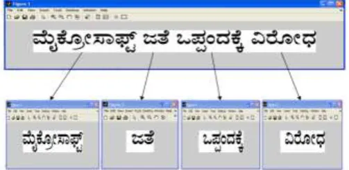
4.2.2 WORD SEPARATION

Word separation is done by taking the vertical projection profile of an input text line. For script, spacing between the words is greater than the spacing between characters in a word. The spacing between the words is found by taking the vertical projection profile of an input text line. The width is more between the words in line as compared to the width that exist between characters in a word. This information is used to separate words from the input text lines. Figure 4.2.2 shows word separation from text line.

Figure 4.2.2: Word separation from text line

4.2.3 BOUNDARY BOX FITTING

[image:2.595.317.553.213.304.2] [image:2.595.308.560.486.609.2]

(3)

[image:3.595.39.285.95.202.2]

(a) (b)

Fig 4.2.3: a) Binarized Image before Boundary Box Fitting

b) After Boundary Box Fitting

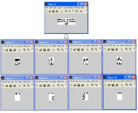
4.3 REGION BASED FEATURE EXTRACTION

Once the image is pre processed then it ready for feature extraction. Here we are dividing the boundary box fitted image into eight equal parts as show in the figure 3.3 (a).

Fig 4.3(a): Dividing image in to eight equal parts.

Each part is a region for feature extraction. Here features are extracted using Haar Discrete Wavelet Transform (Haar DWT). The discrete wavelet transform is a very useful tool for image processing. It decomposes signal into different components in the frequency domain. Two-dimensional discrete wavelet transform (2-D DWT) decomposes an input image into four sub-bands, one average component and three detail components (Horizontal, vertical and Diagonal). Each divided part from the Image is applied to 2-D discrete wavelet transform and output is further considered for feature extraction.

4.4 SCRIPT CLASSIFICATION

This involves developing a suitable Neural Network Model. Artificial neural networks (ANNs) have the ability to learn and classify script by a learning process. Learning vector quantization of ANN is proposed for training and testing. Learning vector quantization (LVQ) is a feed forward neural network used for script classification. It has a superior

performance over back propagation method in the sense of minimizing the classification errors. Features extracted from South Indian Scripts are presented to LVQ-NN which recognizes any one of the four scripts.

4.4.1 TRAINING

Behind successful classification of scripts require training of neural network architecture. The extracted features are presented to LVQ-NN to train. Learning vector quantization (LVQ) networks are used to solve classification problems. The function NEWLVQ takes min and max values for input elements, number of hidden neurons, class percentages, learning rate and learning function. Number of hidden neurons in NEWLVQ is varied based on extracted features for a script. The network is trained for maximum epochs or until the network performance goal met. Flow chart of training phase is shown in figure 4.5.1.

4.4.2 TESTING

Once the Neural Network is trained successfully then it is used for testing to confirm the classification. In testing, input image is selected and its features are extracted and given to the trained model. The trained LVQ – NN model classifies the given sample and recognizes the script. Flow chart for testing phase is shown in the figure 4.5.2.

4.5 FLOW CHART

4.5.1 FLOW CHART OF TRAINIG PHASE

Fig 4.5.1: Training Flow Chart

[image:3.595.42.284.324.523.2] [image:3.595.312.552.460.674.2]

(4)

[image:4.595.100.221.116.270.2]

4.5.2 FLOW CHART OF TESTING PHASE

Fig 4.5.2: Testing Flow Chart

Above figure shows the flow chart of testing phase. Testing phase also carries extraction of features of script images. Script images to be recognized by network are presented to trained network.

5. FEATURES EMPLOYED

5.1 DISCRETE WAVELET TRANSFORM (DWT)

In general wavelet is a small wave function, which is used to transform the signal into frequency bands and also provides information about where that particular frequency is present. The Discrete Wavelet Transform (DWT), which is based on sub-band coding, is found to yield a fast computation of Wavelet Transform. It is easy to implement and reduces the computation time and resources required. DWT is just a sampled version of CWT.

The Continuous Wavelet Transform (CWT) is provided by equation

where x(t) is the signal to be analyzed. ψ(t) is the mother wavelet or the basis function. All the wavelet functions used in the transformation are derived from the mother wavelet through translation (shifting) and scaling (dilation or compression). The mother wavelet used to generate all the basic functions is designed based on some desired characteristics associated with that function. The translation parameter τ relates to the location of the wavelet function as it is shifted through the signal. Thus, it corresponds to the time information in the Wavelet Transform. The scale parameter s is defined as |1/frequency| and corresponds to frequency information. Scaling either dilates (expands) or compresses a signal. Large scales (low frequencies) dilate the signal and provide detailed information hidden in the signal, while small scales (high frequencies) compress the signal and provide global information about the signal. Notice that the Wavelet Transform merely performs the

convolution operation of the signal and the basis function. The above analysis becomes very useful as in most practical applications, high frequencies (low scales) do not last for a long duration, but instead, appear as short bursts, while low frequencies (high scales) usually last for entire duration of the signal. There are a number of basic functions that can be used as the mother wavelet for Wavelet Transformation. Since the mother wavelet produces all wavelet functions used in the transformation through translation and scaling, it determines the characteristics of the resulting Wavelet Transform. Therefore, the details of the particular application should be taken into account and the appropriate mother wavelet should be chosen in order to use the Wavelet Transform effectively.

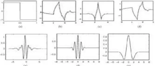
Figure 5.1.a Wavelet families (a) Haar (b) Daubechies4 (c) Coiflet1 (d) Symlet2 (e) Meyer (f) Morlet (g) Mexican Hat.

[image:4.595.309.559.274.380.2]

(5)

[image:5.595.197.555.50.196.2]

This kind of two-dimensional DWT leads to a decomposition of approximation coefficients at level j in four components: the approximation at level j + 1, and the details in three orientations (horizontal, vertical, and diagonal).The following function can be used to decompose a signature image into sub images, which is available in the MATLAB library.

[cA,cH,cV,cD] = dwt2(X,'wname')………..(1)

here X is a 2D signature image, the dwt2 command performs a single-level two-dimensional wavelet decomposition with respect to either a particular wavelet or particular wavelet decomposition filters (Lo_D and Hi_D) you specify.

[cA,cH,cV,cD] = dwt2(X,'wname')…………..(2)

This function computes the approximation coefficients matrix cA and details coefficients matrices cH, cV, and cD (horizontal, vertical, and diagonal, respectively), obtained by wavelet decomposition of the input matrix X. The 'wname' string contains the wavelet name. [cA,cH,cV,cD] = dwt2(X,Lo_D,Hi_D) computes the two-dimensional wavelet decomposition as above, based on wavelet decomposition filters that you specify.

• Lo_D is the decomposition low-pass filter.

• Hi_D is the decomposition high-pass filter.

Lo_D and Hi_D must be the same length.

4.2 FEATURE EXTRACTION USING DWT

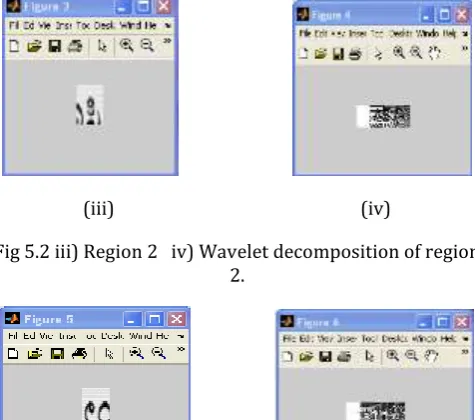
Features are extracted using Haar Discrete wavelet transform (Haar DWT). The discrete wavelet transform is a very useful tool for image processing. It decomposes signal into different components in the frequency domain. Two-dimensional discrete wavelet transform (2-D DWT) decomposes an input image into four sub-bands, one average component and three detail components (Horizontal, vertical and Diagonal). Before feature extraction, input script image is divided into eight equal regions as shown in figure 4.3(a) and for each of the region, first level DWT is applied with the filter called ‘haar’. DWT decomposes each region into four sub-images as shown in the figure below.

(i) (ii)

Fig 5.2 i) Region 1. ii) Wavelet decomposition of region 1.

[image:5.595.314.554.223.339.2]

(iii) (iv)

Fig 5.2 iii) Region 2 iv) Wavelet decomposition of region 2.

(v) (vi)

Fig 5.2 v) Region 3 vi) Wavelet decomposition of region 3.

[image:5.595.315.553.230.440.2]

(vii) (viii)

Fig 5.2 vii) Region 4 iv) Wavelet decomposition of region 4.

(ix) (x)

[image:5.595.316.554.381.485.2] [image:5.595.307.559.512.627.2]

(6)

[image:6.595.40.283.234.490.2]

(xi) (xii)

Fig 5.2 xi) Region 6 xii) Wavelet decomposition of region 6.

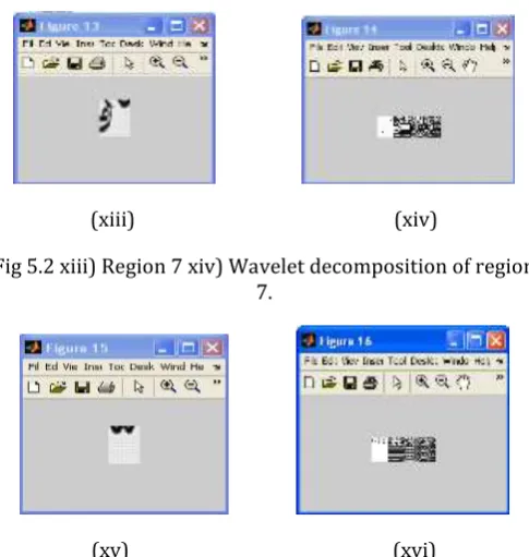
(xiii) (xiv)

Fig 5.2 xiii) Region 7 xiv) Wavelet decomposition of region 7.

[image:6.595.46.279.373.499.2]

(xv) (xvi)

Fig 5.2 xv) Region 8. xvi) Wavelet decomposition of region 8.

Then for each of the detailed coefficient matrices, features such as maximum horizontal projection positions and maximum vertical projection positions are extracted.

5.2.1 MAXIMUM HORIZONTAL PROJECTION POSITION

To compute maximum horizontal projection position, first the number of pixels in each row of region is counted. The row, which has highest pixels value, is taken as maximum horizontal projection position. This position is normalized by dividing it by number of rows which is considered as feature value.

5.2.2 MAXIMUM VERTICAL PROJECTION POSITION

To compute maximum vertical projection position, first the number of pixels in each column of region is counted. The column, which has highest pixels value, is taken as maximum vertical projection position. This position is normalized by dividing it by number of column which is considered as the feature value.

Algorithm 5.2: Step by step process to extract features from script image.

Input: Pre processed image

Output: 24 maximum vertical projection positions, 24 maximum horizontal projection positions.

Start

•Step 1: Read database image from specified location.

•Step 2: Divide the image into 8 blocks as shown in the figure 4.3 (a)

•Step 3: for 1 to 8 blocks do

 Apply 2D-DWT to the region to get 3 detailed coefficient matrices (sub images) using function (1) from section 5.1.

 Calculate maximum horizontal projection position and maximum vertical projection position of 3 sub images as discussed above to get total of 6 features for each region. •Step 4: These 48 parameters are taken as a feature vector for each of the script images and write them in a text file.

Stop

6. LVQ NEURAL NETWORK

6.1 NEURAL NETWORKS

Neural networks are the massively parallel structures of simple processing units, which have a natural propensity for storing experiential knowledge and making it available for use. The true power and advantage of neural networks lies in their ability to represent both linear and nonlinear relationships and to learn these relationships directly from the data being modeled. Neural networks can be used for solving computationally complex tasks such as image processing, computer vision, pattern recognition etc. Neural network models have been applied in low level image processing, image segmentation n-clustering techniques for image coding, image restoration, reconstruction, non linear image filtering, target detection, radar imaging, medical imaging, document analysis, character, and signature, face and object recognition. It has also found applications in three-dimensional object recognition, motion estimation, stereovision and expert systems. The neural network used in this study is “Learning Vector Quantization (LVQ) neural network”. LVQ can be understood as a special case of an artificial neural network, more precisely.

6.2 LEARNING VECTOR QUANTIZATION (LVQ) NEURAL NETWORK.

(7)

divided into two layers. The first layer is competitive layer containing hidden neurons, in which each neuron represents a subclass, the second layer typically linear in which each neuron represents a class. A class may be composed of several subclasses. The second layer combines several subclasses into a class through weight matrix. In the unsupervised Learning Vector Quantization (LVQ), the neighbourhood set contains only the winner node. Such learning rule is called the winner-take all. Learning vector quantization employs a self-organizing network approach, which uses the training vectors to recursively “tune” placement of competitive hidden units that represent categories of the inputs. Once the network is trained, an input vector is categorized as belonging to the class represented by the nearest hidden unit. The hidden units may be thought of as having inhibitory connections between each other so that the unit with the largest input “wins” and inhibits all other units to such an extent that only the winning unit generates an output. In the computer simulation there are no actual inhibitory connections and the winner is simply the hidden unit “closest” to the input vector.

6.2.1 LVQ NETWORK ARCHITECTURE

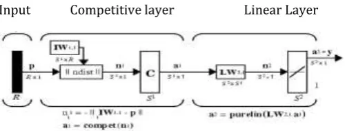
[image:7.595.37.289.400.495.2]

Input Competitive layer Linear Layer

Fig 6.1: architecture of LVQ-NN

Where R= number of elements in the input vector

S1=number of competitive neurons

S2=number of linear neurons

An LVQ network has a first competitive layer and a second linear layer. The linear layer transforms the competitive layer's classes into target classifications defined by the user. The classes learned by the competitive layer are referred to as subclasses and the classes of the linear layer as target classes. Both the competitive and linear layers have one neuron per (sub or target) class. Thus, the competitive layer can learn up to S1 subclasses. The linear layer to form S2 target classes, in turn, combines these. (S1 is always larger than S2).

6.2.2 CREATING AN LVQ NETWORK

LVQ-NN can be created with the function newlvq available in MATLAB Neural Network toolbox.

net=newlvq(PR,S1,PC,LR,LF)………(3)

Where,

 PR is an R-by-2 matrix of minimum and maximum values for R input elements.

 S1 is the number of first-layer hidden neurons.  PC is an S2-element vector of typical class

percentages.

 LR is the learning rate (default 0.01).

 LF is the learning function (default is learnlv1).

6.2.3 TRAINING OF LVQ-NN

Presenting input vectors (features) and adjusting the hidden units based on their proximity to the input vector accomplish training an LVQ network. The nearest hidden unit is moved a distance proportional to the learning rate, toward the training vector if the class of the hidden unit and the training vector match, and away if they do not. The hidden layer weights are trained in this manner for an arbitrary number of iterations, usually with the learning rate decreasing as training progresses. The objective is to place the hidden units so as to cover the decision regions of the training set.

When we run training module using MATLAB toolbox, it will show training neural network window, which consists of LVQ-NN architecture, number of epochs (iterations of presenting input features to adjust the weights), performance goal and time taken to reach that goal. When the training of LVQ-NN is completed, it will show the message “performance goal met”. Training is performed on three experiments as shown in table.

Training set 1:

Number of samples considered for each script: 30

Number of first layer hidden neurons: 40

Learning rate: 0.01

Performance: 0.02

Training set 2:

Learning rate: 0.01

(8)

Learning rate: 0.01

Performance: 0.0222

Figure 6.2(a) shows LVQ NN training window for 75 samples of each Kannada, Telugu, Tamil and Malayalam Script. Figure 6.2(b) shows LVQ NN training window for 50 samples of each Kannada, Telugu, Tamil and Malayalam Script.

Fig 6.2 (a) Training window for 75 samples for each South

Indian Script

Fig 6.2 (b) Training window for 50 samples for each South Indian Script

6.2.4 TESTING USING TRAINED LVQ-NN

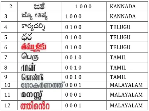
In testing, input image from testing set is selected and its features are extracted and given them to the trained model, the trained LVQ-NN model classifies given sample and recognizes the script. Table shows the result tested for first 3 samples of each south Indian script.

Table 6.2.4: Result analyzed for South Indian script samples.

Sl.

No Script Sample Corresponding output pattern Script type

1 1 0 0 0 KANNADA

2 _{1 0 0 0} KANNADA

3 1 0 0 0 KANNADA

4 0 1 0 0 TELUGU

5 0 1 0 0 TELUGU

6 0 1 0 0 TELUGU

7 0 0 1 0 TAMIL

8 0 0 1 0 TAMIL

9 0 0 1 0 TAMIL

10 _{0 0 0 1} MALAYALAM

11 0 0 0 1 MALAYALAM

12 0 0 0 1 MALAYALAM

7. EXPERIMENT CONDUCTED

Three separate experiments were conducted using the proposed model and results of these are described in this section using graph.

Experiment 1

[image:8.595.304.564.97.290.2] [image:8.595.58.267.277.398.2]

In this experiment, DWT is applied to whole script images, then extracted minimum and maximum horizontal and vertical projection position from script images to get 4*3=12 features. Then this features vector was given to train the LVQ-NN. Accuracy obtained by this experiment was too low (60% to 80%) for 30 to 70 script images as shown in the figure 7.2.a and 7.2.b.

Table 7.2.a: 20 samples for training and 10 samples for testing.

KANNAD

A TELUGU TAMIL MALAYALAM ACCURACY 25/30=8

3% 22/30=73% 27/30=90% 23/30=76% 80%

Fig 7.2.a: Accuracy graph for 30 samples in exp1

Table 7.2.b: 50 samples for training and 20 samples for testing

[image:8.595.61.264.433.552.2] [image:8.595.304.566.514.683.2]

(9)

[image:9.595.327.536.54.198.2]

Experiment 2

[image:9.595.57.279.87.224.2]

In this experiment, another 12 features are added to the feature vector (12+12) obtained in the experiment 1. These 12 features are obtained by dividing the images vertically into two regions, then applying DWT to each of these regions and extracting minimum and maximum horizontal and vertical projection position from each of the sub images. Accuracy obtained by this experiment was improved to 78% to 84% for 30 to 70 script images as shown in the figure 7.2.c and 7.2.d.

Table 7.2.c: 20 samples for training and 10 samples for testing

KANNADA TELUGU TAMIL MALAYALAM ACCURACY

27/30=90

[image:9.595.300.570.400.541.2]

% 21/30=70% 25/30=83% 27/30=90% 84%

Fig 7.2.c: Accuracy graph for 30 samples in exp2.

Table 7.2.d: 50 samples for training and 20 samples for testing

KANNADA TELUGU TAMIL MALAYALAM ACCURACY

59/70=84

% 52/70=74% 57/70=81% 49/70=70% 78%

Fig 7.2.d: Accuracy graph for 70 samples in exp2

Experiment 3

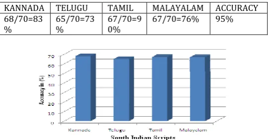
In this experiment, another 24 features are added to the feature vector (24+24) obtained in the experiment 2. These 24 features are obtained by dividing the images vertically into two regions and horizontally into four regions, then applying DWT to each of these regions and extracting maximum horizontal and vertical projection position from each of the sub images. Accuracy obtained by this experiment was improved to 92% to 95% for 70 to 100 script images as shown in the figure 7.2.e and 7.2.f.

Table 7.2.e: 50 samples for training and 20 samples for testing.

KANNADA TELUGU TAMIL MALAYALAM ACCURACY 68/70=83

% 65/70=73% 67/70=90% 67/70=76% 95%

Fig 7.2.e: Accuracy graph for 70 samples in exp3.

Table 7.2.f: 70 samples for training and 30 samples for testing

KANNADA TELUGU TAMIL MALAYALAM ACCURACY 96/100=83

[image:9.595.32.566.409.754.2]

% 91/100=73% 89/100=90% 93/100=76% 92%

[image:9.595.28.294.421.629.2]

(10)

[image:10.595.51.275.152.256.2]

LVQ NN recognizes 92% to 95% of Kannada, Telugu, Tamil and Malayalam South Indian Scripts from 100 samples.

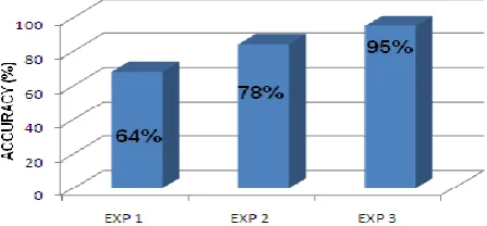
Fig 7.2.g: Overall Accuracy graph of experiments

Above figure shows overall graph of experiment. Experiment 1 with 64%, Experiment 2 with 78% and Experiment 3 with 95 %.

CONCLUSION

In this work, a South Indian script recognition system designed using 3 stages namely pre processing, feature extraction and classification in order to make the right decision is presented. Script recognition of Kannada, Telugu, Tamil and Malayalam is based on 48 wavelet features of different scripts images and the recognizer is LVQ NN. More powerful set of features are derived from wavelet coefficients and one advantages of this LVQ NN algorithm is short computational time. Experimental evidence has shown a method to provide substantial wavelet features. 92% to 95% accuracy is obtained for 70*4 samples used for training LVQ NN. This accuracy can be improved still with the more number of features.

FUTURE WORK

Future work of this project include an analysis of new features of script images and combining those with the feature vector used in this work to obtain better accuracy than the accuracy of present work.

REFERENCES

1. Gopal Datt Joshi, Saurabh Garg, Jayaswami Sivaswamy, “A Generalized Frame Work for Script Identification”. International Journal of Document Analysis and Recognition (IJDAR).

2. S Basavaraj Patil, N V Subbareddy, “Neural Network based System for Script Identification in Indian Document”. Sadhana Vol. 27, Part1, February 2002, pp. 83-97.

3. Huanfeng Ma, aDavid Doermann, “Word Level Script Identification for Scanned Document Images”.

Published Website:

www.lampsrv02.umiacs.umd.edu.

4. M C Padma, Dr P A Vijaya, “Language Identification of Kannada, Hindi and English words through Visual Discriminating Features”. International Journal of Computational Intelligence System, Vol.1, No.2 (May, 2008), 116-126.

5. B V Dhandra, Mallikarjuna Hangarge, “Global and Local Features Based Handwritten Text Words and Numerical Script Identification”. International Conference on Computational Intelligence and Multimedia Applications 2007.

6. Sukalpa Chanda, Srikant Pal, Umapada Pal, “Word-wise Sinhala Tamil and English Script Identification Using Gaussian Kernel SVM”. IEEE SOCIETY 978-1-1-4244-2175-6/08

7. Shamik Sural, P.K.Das, “Recognition of an Indian Script using Multilayer Perceptrons and Fuzzy Features”. Sixth International Conference on Document Analysis and Recognition (ICDAR2001), Seattle, 2001, pp. 1120-1124.

8. Ranjith Kumar, Vamsi Chaitanya, C. V. Jawahar, “A Novel Approach to Script Separation”. Published Website: www.cvit.iiit.ac.in-papers-ranjith03novel

9. Sukalpa Chanda, Srikanta Pal, Katrin Franke, Umapada Pal, “Two-stage Approach for Word-wise Script Identification”. 2009 10th International Conference on Document Analysis and Recognition.

10. Gopal Datt Joshi, Saurabh Garg, Jayanthi Sivaswamy, “Script Identiﬁcation from Indian Documents”. Springer-Verlag Berlin Heidelberg 2006, LNCS 3872, pp. 255–267.

11. K. Roy, U. Pal, “Word-wise Hand-written Script Separation for Indian Postal automation”. Published Website: www.hal.archives-ouvertes.fr

12. S.Abirami, Dr. D.Manjula, “A Survey of Script Identification techniques for Multi-Script Document Images”. International Journal of Recent Trends in Engineering, Vol. 1, No. 2, May 2009.

13. Guo Xian Tan, Christian Viard-Gaudin, Alex C. Kot, “Information Retrieval Model for Online Handwritten Script Identification”. 2009 10th International Conference on Document Analysis and Recognition.

(11)

Reconstruction for Word Level Script Identification”. Published Website: www.cscjournals.org.

16. ” Lijun Zhou, Yue Lu, Chew Lim Tan, “Bangla/English Script Identification Based on Analysis of Connected Component Profiles”. Published Website: www.comp.nus.edu.

17. Dileep Kumar, “AI Approach to Hand Written Devnagiri Script Recognition” .TENCON '91.1991 IEEE Region 10 International.

18. Ahmad A R, Viard Gaudin C, Khalid M, “Lexicon-based Word Recognition Using Support Vector Machine and Hidden Markov Model”. 2009 10th International Conference on Document Analysis and Recognition.

19. Andrew Busch, Wageeh W Boles, Sridha Sridharan, “Texture for Script Identification”.

20. IEEE Transactions on Pattern Analysis and Machine Intelligence, vol. 27, no. 11, November 2005.