Towards Evolving Cooperative Mapping for Large Scale UAV Teams

Towards Evolving Cooperative Mapping for

Large-Scale UAV Teams

Elnaz Shafipour Yourdshahi, Plamen Angelov, Leandro Soriano Marcolino, Georgios Tsianakas

Lancaster University Lancaster, UK

{elnaz.shafipour, p.angelov, l.marcolino, g.tsianakas}@lancaster.ac.uk

Abstract—A team of UAVs has great potential to handle real-world challenges. Knowing the environment is essential to perform in an effective manner. However, in many situations, a map of the environment will not be available. Additionally, for autonomous systems, it is necessary to have approaches that require little energy, computing, power, weight and size. To address this, we propose a light-weight, evolving, and memory efficient cooperative approach for estimating the map of an environment with a team of UAVs. Additionally, we present proof-of-concept experiments with real-life flights, showing that we can estimate maps using an off-the-shelf web-camera.

I. INTRODUCTION

A team of Unmanned Aerial Vehicles (UAVs) has a great potential for tackling real-world challenges [1], such as localising victims in disaster scenarios [2] or patrolling a specified area [3]. The use of multiple UAVs allows the task to be executed faster, and in a fault-tolerant manner, as the loss of a single unit will not necessarily cause the failure of the full system.

However, in order to adequately perform in a mission, team members must have the current map of the environment. The map can be used by each robot to estimate its own localisation, and also for planning joint actions towards solving some given mission. Additionally, it is desirable to have large-scale teams, for great efficiency and fault tolerance.

Simultaneous localisation and mapping (SLAM) is a very active topic of research. Many works use range-based devices, such as RGB-D cameras, or laser rangefinders, in order to find landmarks or relevant scene features [4], [5], while integrating motion estimations given by an Inertial Measurement Unit (IMU). A feedback loop is also commonly employed to further improve localisation estimation, for instance using variations of the Kalman Filter [6].

Given a UAV team, it is natural to think about cooperative SLAM approaches, since the maps of multiple robots can be merged [7]. Similarly to the single robot case, point clouds or stereo cameras are used for landmark identification, and common landmarks across the local maps must be identified in order to merge multiple maps into a common global map (for instance, using the RANSAC algorithm) [8], [9]. These methods, however, are expensive, as they require specialised sensors, and the landmark identification and aggregation is costly. Therefore, more light-weight approaches would be desirable for large scale robotics.

Hence, in this paper, we propose a light-weight, memory-efficient, evolving approach for landmark identification and map aggregation, based on the Recursive Density Estimation (RDE) [10], [11] method. We also demonstrate how this approach can be applied when estimating landmarks in real-time by real UAVs. We aggregate the estimated maps of multiple UAVs in an on-line manner, with no pre-training nor central controller. Furthermore, we build an experimental UAV platform using a commodity web-camera, and we present our proof-of-concept experiments including aggregating the estimated maps of two real UAVs.

II. RELATEDWORKS

Landmark-based mapping and navigation is a common technique in robotics [12]–[14], since it allows for navigation in previously unknown, and unstructured environments. However, previous work assumed simple landmarks artificially placed in the environment (e.g., bar-codes in Busquets et al. (2003) [12]), or assumes a database of potential landmarks (e.g., [13]). Other works, such as Trahanias et al. (1999) [14], do not assume a landmark database, but the system must be pre-trained for a specific environment.

Recent work assumes robots equipped with range-based sensors, and identify scene features from point clouds [4], using the SURF method [15]. A non-linear optimisation based approach has also been employed [5], in order to integrate information from an Inertial Measurement Unit (IMU) with seen features detected from stereo camera images, using the BRISK approach [16]. Additionally, a low-cost platform for visual odometry in UAVs has also been recently proposed, using an IMU and a single camera [17], but they focus on precise movement estimation, instead of mapping.

Fig. 1: Dividing a frame into bins to calculate the density (from [11]).

On the other hand, some works on cooperative mapping focus on how to best plan the trajectory of each individual robot, sometimes assuming that common landmarks across maps would be easily identified [19], or relying on very accurate relative positioning systems for map aggregation [20].

Alternatively, in this work, we propose a light-weight, and memory efficient approach for cooperative mapping, which would be more appropriate for autonomous UAVs, without requiring expensive sensors and costly algorithms. Our main contribution is to show that we can use an evolving recursive algorithm for landmark identification and map aggregation, building upon the Recursive Density Estimation (RDE) ap-proach [10], [11].

III. METHODOLOGY

A. Automatic Landmark Detection

We developed our technique for landmark detection by extending our previous work [10], [11], where Recursive Density Estimation (RDE) was introduced for automatically detecting landmarks from front-view cameras. The only inputs for RDE are the stream of images from a camera, no pre-training and no human involvement is required. We will present a summary of the previous method, before introducing our approach.

First, we divide a frame ofM×N pixels into smaller local images, or bins (Figure 1). The mean value of the colour of all pixels included in each bin is calculated for each of the three colour channels: Red, Green, and Blue. The resulting mean will represent each bin. Then, we compute the colour density of the whole frame based on the following equation [10]:

D(sk) = 1

1 +||sk−µk||2+Sk− ||µk||2

,

where D denotes density; sk =

[R1_k, G1_k, B_k1, . . . , R_ki, Gi_k, B_ki]T represents the vector of the mean value of the pixels in RGB form of the frame number k, for each bin i. Sk denotes the scalar product of

the values in the specified colour vector , and µk is the mean

value of the vectors (across the frames, from the beginning of the video until the current frame k).

Fig. 2: Density evolution within the video stream (from [11]).

Both the mean,µk, and the scalar product,Sk, are updated

recursively, as follows [10]:

µk =

k−1

k µk−1+

1

ksk, µ1=s1 Sk=

k−1

k Sk−1+

1

k||sk||

2_{, S}

1=||s1||2

Similarly, having the value of the density updated for the currentk-th frame, we can also calculate and update the mean density (D¯k) and the standard deviation of the density (σkD)

recursively, as follows [10]:

¯

Dk =

k−1

k

¯

Dk−1+

1

kDk,

¯

D1=D1

(σD_k)2=k−1

k (σ

D k−1)

2₊1

k(Dk−

¯

Dk)2,(σD₁)2= 0

Hence, the calculation of the density, and its mean and standard deviation, keeps being updated at each new frame of the given video, and it is not required to keep the full history of previous frames. Figure 2 shows a sample result of the above calculations, which demonstrate the density of each frame grabbed by the input video as well as the mean density minus the standard deviation (mean(D)−std(D)). The frames for which the value of density drops below the value of mean(D)−std(D)are denoted as a landmark. We show in the figure pictures of two landmarks against their density.

B. The proposed new approach

Fig. 3: Considering each bin as a frame, and dividing it into bins.

We assume a set of UAVs, each equipped with a local IMU, and its own ground-facing camera. We consider that the cameras are all directly facing the ground. Additionally, each UAV may start at any arbitrary position, and it will use the IMU to keep track of its position in relation to its starting location. In this paper, we focus on a light-weight landmark identification and map aggregation. Therefore, we do not employ a feedback loop (e.g., Kalman Filter [6]) for further improving the position estimation beyond the IMU data, although this could be easily added to our approach. We will first describe our landmark identification technique, and afterwards, we will describe the map aggregation across UAVs.

In order to have a more precise landmark detection from a top view, each bin will be considered as a “frame” and it will be further divided to another level of bins, which is shown in Figure 3 with blue colour. Hence, the density value will now be calculated for each bin, and the evaluation is performed for each bin across frames. Note, again, that although we compare for each bin across the frames, we do not need to store the history of the previous frames per bin, as we use the recursive calculations above, which require only the current frame and the current density information. If the technique identifies a landmark in one of the bins, we save the full framewhere the bin is contained as a new landmark.

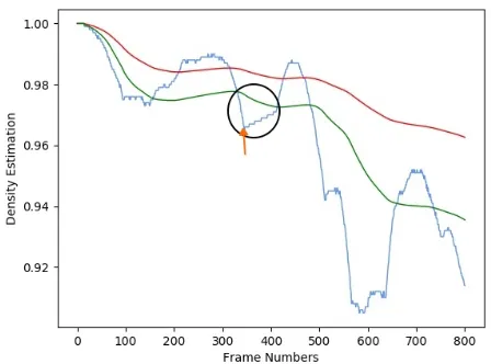
Additionally, we find the minimum value of each density “drop”. We define the “drop” when the density falls below its standard deviation until it goes back again to be within the standard deviation. Therefore, for each drop of the density, we select a single landmark, which has the minimum density at that drop section. An example of a drop is shown in Figure 4, where the black circle shows the location of the drop and the orange arrow represents the frame that is selected as a new landmark.

1) Filtering Landmarks: After automatically selecting land-marks with the proposed approach, we noticed that there are still landmarks which are similar to each other. Therefore, we filter similar landmarks by analysing the colour histograms.

A colour histogram is a vector where each entry stores the number of pixels of a given colour in the image [21]. We

Fig. 4: Example of a density drop within the black circle and the selected landmark with the orange arrow. The blue line shows the current density, the red line shows its average, and the green line shows its standard deviation.

generate one histogram vector for each landmark image, and perform pair-wise comparisons across all of them. We use the correlation between two histograms as a similarity metric. That is, given the histograms of two potential landmarks,H1,H2, the similarity between them will be given by:

d(H1, H2) = P

I(H1(I)−H¯1)(H2(I)−H¯2)

q P

I(H1(I)−H¯1)2PI(H2(I)−H¯2)2

, (1)

where H¯k = _N1 PIHk(I), and N is the total number of

histogram bins.

If the result of the comparison of two images is higher than a given threshold, we assume that they are the same, and we select just one of them as a landmark. We will use a similar process in order to find common landmarks across multiple UAVs, in order to merge their maps, as we will describe later. 2) Calculating positions from IMU: Besides selecting land-marks, we also need to process the IMU data, in order to find the estimated position of the selected landmarks. Hence, each UAV must use the IMU to estimate its current position in relation to its starting point.We perform this estimation based on the following steps:

1) Initialise current position and current velocity to 0:

Pc= 0

Vc= 0

2) Calculate timeT as the difference of two time stamps (the current and the previous time stamp);

3) Calculate velocity based on following the formula, where

V =Vc+A·t;

4) Calculate position based on the following formula:

P =Pc+V ·t+ 1 2A·t

2

5) Finally, update current position and velocity by latest calculated values:

Pc=P

Vc=V

6) The same calculations are performed for estimating the

x,y andz positions.

3) Merging Multiple Maps: As we have multiple UAVs, which may have started from different locations, we need to merge their estimated maps in order to have a single global map.

Let us consider n sets of points fornUAVs, where each point represents an estimated landmark by the corresponding UAV. As the flights started from different locations, their (0,0,0) points are different (i.e., they correspond to different positions in a “global” frame). Therefore, we haven different Cartesian Coordinate Systems, one for each UAV. In order to have a common map, we need to have the points in a single Cartesian Coordinate System. We use the method presented in [22] in order to align the Cartesian Coordinate Systems.

That is, we assume that each time two UAVs meet, they are going to exchange their local estimated maps, and aggregate their own map with the one received from the neighbour. Hence, to have one Cartesian Coordinate System, we need to find a rotation and a translation between the two sets of corresponding point data.

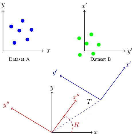
As it is shown in Figure 5 there are two datasets in the two coordinate systems: Dataset A and Dataset B. We indicate the corresponding points across both datasets with the same colour. Let Rbe the rotation, andT the translation required to align the coordinate systems. We need to solve forR andT in the equation below:

B=R×A+T

Finding the optimal rigid transformation matrix can be broken down into the following steps:

1) Find the centroids of all of the datasets,

2) Bring all of the datasets to the origin, then find the optimal rotation (matrixR),

3) Find the translationT

We used the above technique and assumed the position of common landmarks as the corresponding points across both datasets. We analyse the colour histograms in order to estimate common landmarks across UAVs, similarly to how we filtered repeated landmarks in the same local map. That is, we compare each landmark found by one UAV against all the landmarks found by another UAV. LetH1be the histogram of a landmark

y

x

Dataset A

y

x

Dataset B

x

y

y

x

R

T

x

y

Fig. 5: Rotation and translation of two Cartesian Coordinate Systems

in the local map of a UAV, and H2 be the histogram of a landmark in the map of another UAV. We estimate the similarity between both landmarks using Equation 1. If the estimated similarity is above a certain threshold, we assume that they correspond to the same landmark. Finally, we can then convert all local landmarks positions by usingR and T to the second UAV’s Coordinate System.

IV. RESULTS

A. Hardware Platform

We used the DJI S800 Evo Hexacopter UAV in our experiments (Figure 6 (a)). As mentioned, our approach can work with very small and simple hardware. Hence, we only use a single web camera for video data acquisition. We use a commodity web camera: the Logitech QuickCam 5000, shown in Figure 6 (b), which allows only 640x480 pixels resolution. Additionally, we add to the UAV a PixHawk flight controller, for obtaining IMU data (Figure 6 (c)), and an onboard embedded computing board to process the video and IMU data in real-time. Additionally, the UAV is set up with its own independent flight controller, such that video and IMU data acquisition and processing do not interfere with normal flight operations.

B. Experiments

(a) DJI S800 Evo Hexacopter UAV which is capable of flying the data acquisition components.

(b) Logitech QuickCam 5000 used for gathering the video data.

(c) Pixhawk 2.4.8 flight controller used to obtain the IMU data.

Fig. 6: Hardware used in the real life experiments.

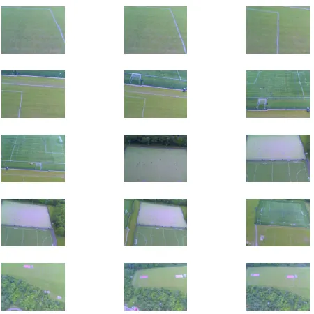
Fig. 7: Filtered landmarks identified by the first UAV.

section, we will show the local map estimation, and final map aggregation of two UAVs1.

Our flights were conducted over the sports fields of Lancaster University. There was a sufficient number of obstacles and ground markings such that it did not just look like grass and green fields for the entirety of the videos. Due to the flight duration limitations (approximately 14 minutes max), each video was 6 minutes in length. The videos showing our real-life flights are available at:

• First UAV: https://drive.google.com/drive/u/0/folders/ 1uAc8GWwemOU4wX7UzhdGkWnR9uPlJ5LV

• Second UAV: https://drive.google.com/drive/u/1/folders/ 1uAc8GWwemOU4wX7UzhdGkWnR9uPlJ5LV

In Figure 7 we show the landmarks identified by the first UAV, after filtering; while in Figure 8 we show the landmarks identified by the second UAV, also after filtering. As we can see, we could find a reasonable number of landmarks from short 6 minutes long flights, and they do not look overly similar to each other.

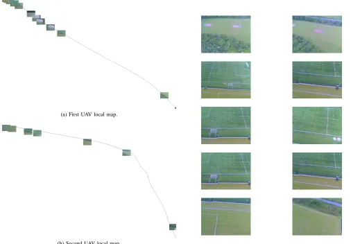
Using these landmarks, each UAV is able to build its local map. In Figure 9 (a) we show the estimated map of the first UAV, while in Figure 9 (b) we show the estimated map of the second UAV. We position the landmark image in the corresponding estimated location of the landmark. Additionally, the blue line shows the estimated trajectory of the UAV.

Finally, each UAV can build the combined map. For aggregating both maps, first, each UAV retrieves the landmarks of the other UAV with their positions in their reference frame. Then, all local landmarks are compared with the landmarks of

1_{In order to simulate the aggregation across two UAVs, we actually}

Fig. 8: Filtered landmarks identified by the second UAV.

(a) First UAV local map.

(b) Second UAV local map.

Fig. 9: Created map and trajectory of each UAV.

the other UAV, by analysing the correlations across the colour histograms. For example, we show the similarity results found in our flights in Table I. In Figure 10, we show the landmarks that were considered as common across the flights of both UAVs.

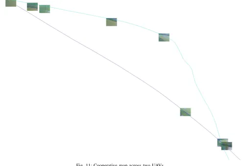
Using these common points across both maps, each UAV finds optimal rotation R and translation T transformation matrices, as described previously. Based on this information, it

373 769 853 1576 2178 263 0.71 0.05 0.01 0.79 0.06 484 0.31 0.27 0.02 0.43 0.04 683 0.01 0.81 0.62 0.09 0.11 832 0.03 0.66 0.39 0.12 0.15 1336 0.01 0.04 0.02 0.02 0.1 1640 0.02 0.01 0.06 0.04 0.11 1865 0.06 0.05 0.08 0.05 0.11 2046 0.07 0.08 0.05 0.08 0.14 2368 0.22 0.41 0.14 0.3 0.14 4170 0.44 0.18 0.26 0.17 0.37 4543 0.33 0.25 0.28 0.2 0.5 4590 0.15 0.15 0.19 0.12 0.69

TABLE I: Comparison value of selected landmarks for both UAVs. The first row shows the first UAV’s frame numbers, and the first column shows the second UAV’s frame numbers.

Fig. 10: Common landmarks across the local maps of the first UAV (first column) and the second UAV (second column).

Fig. 11: Cooperative map across two UAVs.

V. CONCLUSION

Cooperative mapping is fundamental for using UAV teams in real-world tasks, where the environment may not be known in advance. In this paper, we present a light-weight, and memory efficient approach for cooperative mapping. That would allow our approach to be used in real-time.

Our technique is a based on the RDE approach, adapted for identifying landmarks from top-view cameras. Additionally, we show how the landmarks can be filtered, and how the local maps of multiple UAVs can be aggregated into a single global map.

We present proof-of-concept experiments, performing real flights at Lancaster University. In our experiments, we used a UAV equipped with only one simple webcam, but we could still estimate landmark-based maps, and aggregate them into a final common map.

VI. ACKNOWLEDGMENTS

This work was funded by the Defence Science and Technology Laboratory (DSTL), contract reference DSTLX1000110033. We would also like to thank Dr Gruff Morris for his help with the real world UAV flights.

REFERENCES

[1] P. Angelov,Sense and Avoid in UAS: Research and Applications. John Wiley and Sons, 4 2012.

[2] J. Scherer, S. Yahyanejad, S. Hayat, E. Yanmaz, T. Andre, A. Khan, V. Vukadinovic, C. Bettstetter, H. Hellwagner, and B. Rinner, “An autonomous multi-UAV system for search and rescue,” inProceedings of the 13th International Conference on Mobile Systems, Applications, and Services (ACM), 2015.

[3] E. Yanmaz, “Connectivity versus area coverage in unmanned aerial vehicle networks,” inIEEE ICC 2012 Conference Proceedings, 2012. [4] P. Lourenc¸o, B. J. Guerreiro, P. Batista, P. Oliveira, and C. Silvestre,

“Simultaneous localization and mapping for aerial vehicles: a 3-D sensor-based GAS filter,”Autonomous Robots, vol. 40, no. 5, pp. 881–902, Jun 2016.

[5] S. Leutenegger, S. Lynen, M. Bosse, R. Siegwart, and P. Furgale, “Keyframe-based visualinertial odometry using nonlinear optimization,”

The International Journal of Robotics Research, vol. 34, no. 3, pp. 314– 334, 2015.

[6] R. E. Kalman, “A new approach to linear filtering and prediction problems,”Transactions of the ASME–Journal of Basic Engineering, vol. 82, no. Series D, pp. 35–45, 1960.

[7] D. Fox, J. Ko, K. Konolige, B. Limketkai, D. Schulz, and B. Stewart, “Distributed multirobot exploration and mapping,”Proceedings of the IEEE, vol. 94, no. 7, pp. 1325 – 1339, 2006.

[8] J. Dong, E. Nelson, V. Indelman, N. Michael, and F. Dellaert, “Distributed real-time cooperative localization and mapping using an uncertainty-aware expectation maximization approach,” inProceedings of the 2015 IEEE International Conference on Robotics and Automation (ICRA), 2015. [9] A. Cunningham, K. M. Wurm, W. Burgard, and F. Dellaert, “Fully

[10] R. Ramezani, P. Angelov, and X. Zhou, “A fast approach to novelty detection in video streams using recursive density estimation,” in

Intelligent Systems, 2008. IS’08. 4th International IEEE Conference, vol. 2. IEEE, 2008, pp. 14–2.

[11] P. Sadeghi-Tehran, S. Behera, P. Angelov, and J. Andreu, “Autonomous visual self-localization in completely unknown environment,” in Pro-ceedings of the IEEE Conference on Evolving and Adaptive Intelligent Systems (EAIS), 2012.

[12] D. Busquets, C. Sierra, and R. L. de M`antaras, “A multiagent approach to qualitative landmark-based navigation,”Autonomous Robots, vol. 15, no. 2, pp. 129–154, Sep 2003.

[13] R. Murrieta-Cid, C. Parra, and M. Devy, “Visual navigation in natural environments: From range and color data to a landmark-based model,”

Autonomous Robots, vol. 13, no. 2, pp. 143–168, Sep 2002.

[14] P. E. Trahanias, S. Velissaris, and S. C. Orphanoudakis, “Visual recogni-tion of workspace landmarks for topological navigarecogni-tion,”Autonomous Robots, vol. 7, no. 2, pp. 143–158, Sep 1999.

[15] H. Bay, A. Ess, T. Tuytelaars, and L. V. Gool, “Speeded-up robust features (SURF),”Computer Vision and Image Understanding, vol. 110, no. 3, pp. 346–359, 2008.

[16] S. Leutenegger, M. Chli, and R. Y. Siegwart, “BRISK: binary robust invariant scalable keypoints,” inProceedings of the IEEE International Conference on Computer Vision, 2011.

[17] A. Santamaria-Navarro, G. Loianno, J. Sol`a, V. Kumar, and J. Andrade-Cetto, “Autonomous navigation of micro aerial vehicles using high-rate and low-cost sensors,”Autonomous Robots, vol. 42, no. 6, pp. 1263–1280, Aug 2018.

[18] M. Fischler and R. Bolles, “Random sample consensus: a paradigm for model fitting with application to image analysis and automated cartography,”Communications of the ACM, vol. 24, 1981.

[19] V. Indelman, “Cooperative multi-robot belief space planning for au-tonomous navigation in unknown environments,”Autonomous Robots, vol. 42, no. 2, pp. 353–373, Feb 2018.

[20] R. G. Colares and L. Chaimowicz, “The next frontier: Combining informa-tion gain and distance cost for decentralized multi-robot explorainforma-tion,” in

Proceedings of the 31st Annual ACM Symposium on Applied Computing, 2016, pp. 268–274.

[21] P. K. Sahoo, S. Soltani, and A. K. Wong, “A survey of thresholding techniques,”Computer vision, graphics, and image processing, vol. 41, no. 2, pp. 233–260, 1988.