Functional Interpretation of
High-Throughput Sequencing Data
by
Chee Lee
A dissertation submitted in partial fulfillment of the requirements for the degree of
Doctor of Philosophy (Bioinformatics) in the University of Michigan
2016
Doctoral Committee:
Associate Professor Maureen A. Sartor, Chair Professor Margit Burmeister
Assistant Professor Maria E. Figueroa Assistant Professor Stephen C.J. Parker Assistant Professor Indika Rajapakse
©
Chee Lee 2016 All Rights Reservedii
Dedication
iii
Acknowledgements
I would like to thank my advisor, Dr. Maureen Sartor, for her abiding and positive mentorship. She has taught me how to approach research problems from points of views that I have never considered, and provided guidance whenever I needed it. She always has an open door, and is extremely dedicated to the success of her students. Her style of mentorship has inspired a fun yet productive atmosphere in our lab. I have been very fortunate to find such a wonderful mentor for the last 5+ years.
Next I would like to thank my committee members, past and present, for sharing their expertise and enduring through long, often difficult to schedule, committee
meetings. I did my first research rotation with Dr. Margit Burmeister, and years later chose her to be on my committee because her ability to quickly identify computational and biological connections. She did not disappoint in doing the same during all my meetings. Dr. Jim Cavalcoli was an expert in sequencing technologies and provided helpful advice for the sequencing problems that we tackled. Dr. Ken Figueroa was often the one in meetings who would anchor us computational biologist from diverging too far into the technical side. She provided a much needed perspective on the practicality and biological usefulness of my research. Dr. Stephen Parker was always excited about my researcher from the first day I met him during a student luncheon for his faculty
interview. I am very grateful he was able to join my committee and share his experience with gene set enrichment testing and repetitive elements. Dr. Indika Rajapakse always has a smile on his face and the ability to think outside of the box. His expertise in genome organization has helped inspire many ideas in this dissertation.
I would also like to acknowledge additional bioinformatics faculty and staff members. Thank you to Dr. Brian Athey, Dr. Dan Burns, and additionally thanks to Dr. Margit Burmeister for their academic and personal advising. Their dedication to the success of the students in the department goes beyond what is asked of them. Thank
iv
you to Dr. Alla Karnovsky, with whom I did a research rotation with, for serving on my prelim committee and also providing valuable career guidance. I would also like to thank Dr. Tricia Wittkopp, and additional thanks to Dr. Dan Burns and Dr. Indika Rajapakse for also serving on my prelim committee. My prelim committee was critical to providing direction in the scientific process, which ultimately made me a better researcher. Thank you to Dr. Jeff de Wet for being a great teacher and introducing more programming languages to me. My success in the program will also not be possible without the help of all the bioinformatics staff. In particular I would like to thank Julia Eussen for handling all the paperwork, scheduling, and all things behind-the-scenes so seamlessly that we didn’t even notice it was being done. The same goes to Alex Terzian, Aaron Bookvich, and Paul Trombley who has helped set up all of our technology needs from AV
equipment to poster printing and designing graphics for our web apps. Also thanks to Terry Weymouth for helping us develop our websites for our various gene set
enrichment programs.
I have been very fortunate to find a nourishing, fun, and positive research lab. Again I would like to thank Maureen, as well as all Sartor Lab members past and present for creating an environment where we helped each other and were involved in each’s other successes. Thank you to Yanxiao Zhang, Raymond Calvalcante, Snehal Patil, Julie Kim, Yongseok Park, Yu-Hsuan Lin, Lada Koneva, Pelle Hall, Shama Virani, Chris Lee, and Yidan Liu for your friendships and research camaraderie.
My experience in graduate school has also been shaped by my classmates and my friends. From the bioinformatics and biostatistics departments, I want to thank Yanxiao Zhang, Ellen Schmidt, Tom Wolfe, Alex Schmidt, Ryan Welch, Paul Imbriano, and Lee Sam for working alongside me in class projects, helping me with coding when I needed it, and for being great research buddies. My friends whom I met in Michigan: Ariell, Kathryn, Esha, Elizabeth, Kaitlyn, and Purvi - we have kept each other sane all these years. My close friends in MN whom I miss dearly: Meredith, Rachel, Jenna, Brittany, Joe, Andy, Dave, and Chris. Thank you so much for your friendships. My companion, Jonathan Las Fargeas, thank you for being there for me, your infectious energy helps keep my spirits up.
v
Finally I would like to thank my family: my dad, Nao Bee, my mom, Na, and my sisters: Mai Tong, Dia, Mai Song, and my brothers: Touko, Muachi, Teng, and
vi
Table of Contents
Dedication ...ii
Acknowledgements ... iii
List of Figures ... x
List of Tables ... xiii
List of Abbreviations ...xv Abstract ... xvii Introduction ... 1 Chapter 1 1.1 Introduction ... 1 1.2 Background ... 2 1.2.1 High-throughput technologies ... 2
1.2.2 Gene set enrichment testing ... 4
1.3 Overview of dissertation ... 7
ChIP-Enrich: Gene set enrichment testing for ChIP-seq data ... 10
Chapter 2 2.1 Introduction ... 10
2.2 Materials and Methods ... 12
2.2.1 Experimental ChIP-seq peak datasets ... 12
2.2.2 Gene loci definitions and presence of peaks in a locus ... 12
2.2.3 Gene Ontology terms ... 13
2.2.4 Overdispersion test of peak count (given locus length) in each gene set .. 13
2.2.5 Mappability calculations ... 14
2.2.6 ChIP-Enrich method ... 14
2.2.7 R package and website ... 16
2.2.8 Fisher’s exact test for gene set enrichment testing of ChIP-seq data ... 17
2.2.9 Binomial test for GO term enrichment testing of ChIP-seq data ... 17
2.2.10 Permutations to create ENCODE ChIP-Seq data with no biological enrichment ... 17
vii
2.2.11 GRα analysis ... 18
2.3 Results ... 19
2.3.1 Observed relationship between gene locus length and presence of at least one peak in ENCODE ChIP-seq datasets ... 19
2.3.2 ChIP-Enrich method ... 20
2.3.3 Comparison of ChIP-Enrich, Fisher’s exact test and the binomial test for permuted and non-permuted ENCODE datasets ... 21
2.3.4 Influence of locus definition on detection of gene set enrichment ... 23
2.3.5 ChIP-Enrich analysis of the glucocorticoid receptor α (GRα) ... 25
2.4 Discussion ... 26
2.5 Supplementary Methods ... 29
2.5.1 Testing for enriched GO terms with genes of longer (or shorter) than average locus length ... 29
2.5.2 Testing for enriched GO terms with genes having higher or lower than average mappability ... 29
2.5.3 Simulation and enrichment testing of data under the null hypothesis of no GO term enrichment ... 29
2.5.4 GREAT testing on permuted ChIP-seq datasets ... 30
2.6 Supplementary Results ... 31
2.6.1 Effect of locus length and read mappability on gene set enrichment tests 31 2.6.2 Comparison of ChIP-Enrich, Fisher’s exact test, and the binomial test under the null hypothesis of no enrichment using simulated data ... 32
2.6.3 Test behaviors in the presence of overdispersion of peak counts among genes, given locus length ... 33
2.6.4 Slight deflation in p-values compared to what is expected under the null .. 34
2.6.5 Sensitivity analysis for GR ... 34
2.7 Figures ... 35
2.8 Tables ... 39
2.9 Supplementary Figures ... 42
2.10 Supplementary Tables ... 53
Enrich: A cut-off free functional enrichment testing method for RNA-Chapter 3 seq with improved detection power ... 59
viii 3.2 Methods ... 60 3.2.1 Model ... 60 3.2.2 Datasets ... 61 3.2.3 Description of Permutations ... 61 3.2.4 Performance Comparison ... 62 3.2.5 Other comparisons ... 63
3.3 Results & Discussion ... 63
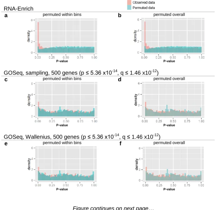
3.3.1 Method performance with permutated data ... 63
3.3.2 Method performance with experimental results ... 64
3.4 Figures and Tables ... 65
Transposons, segmental duplications, sequence mappability, and gene Chapter 4 length: Deciphering their relationship with gene function ... 77
4.1 Introduction ... 77
4.2 Methods ... 81
4.2.1 Locus regions ... 81
4.2.2 Mappability calculations ... 82
4.2.3 Repetitive elements and segmental duplications ... 82
4.2.4 Contribution of repetitive elements and segmental duplications to mappability ... 83
4.2.5 Gene set enrichment testing ... 83
4.2.6 Clustering ... 83
4.2.7 Motif discovery and mappability ... 84
4.3 Results ... 84
4.3.1 Mappability varies by read length and region of gene ... 84
4.3.2 Mappability of repetitive elements and their distribution across genic regions ……….85
4.3.3 Repetitive elements and overall mappability in both genic and regulatory regions are associated with gene function and locus length ... 87
4.3.4 Comparison of mouse and human mappability and locus length ... 90
4.3.5 Effect of mappability on ChIP-seq peak detection ... 91
4.4 Discussion ... 91
ix
Conclusions & Future Directions ... 113
Chapter 5 5.1 Conclusions... 113 5.2 Future Directions ... 116 5.2.1 Chapter 2 ... 116 5.2.2 Chapter 3 ... 117 5.2.3 Chapter 4 ... 118 Bibliography ... 120
x
List of Figures
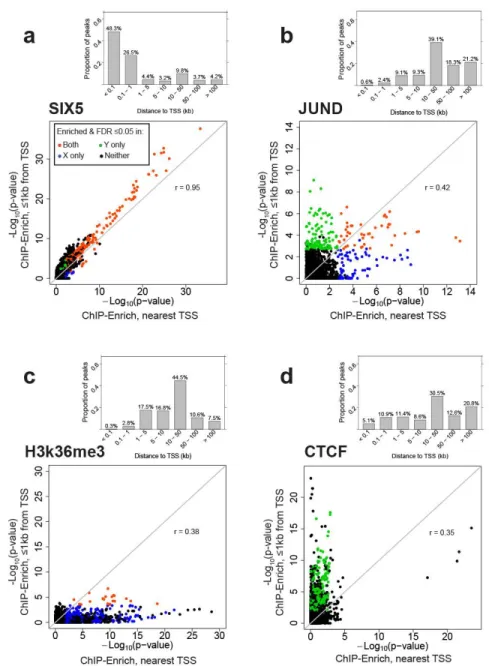
FiguresFigure 2.1 Gene locus length-to-peak presence relationship becomes stronger as total number of peaks increases... 35 Figure 2.2. Overview of ChIP-Enrich ... 36 Figure 2.3. Representative plots of the 4 patterns of enrichment comparing the ≤1kb
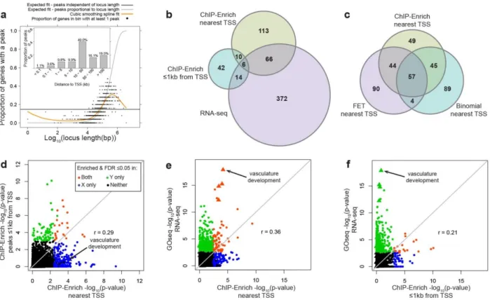
from TSS and nearest TSS locus definitions. ... 37 Figure 2.4 Comparison of GRα enrichment results for ChIP-seq (using two locus
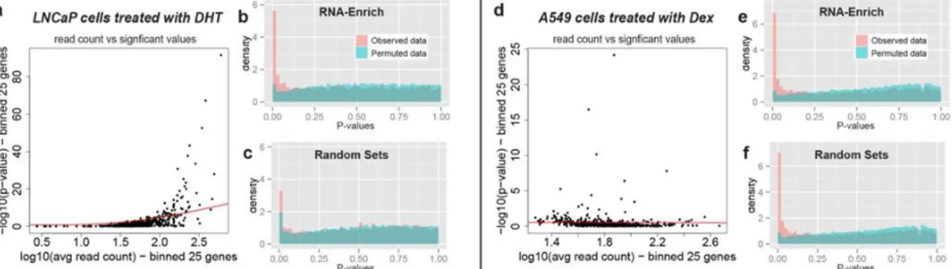
definitions) and RNA-seq data from A549 cells ... 38 Figure 3.1. Comparison of RNA-Enrich with random sets with two datasets exhibiting
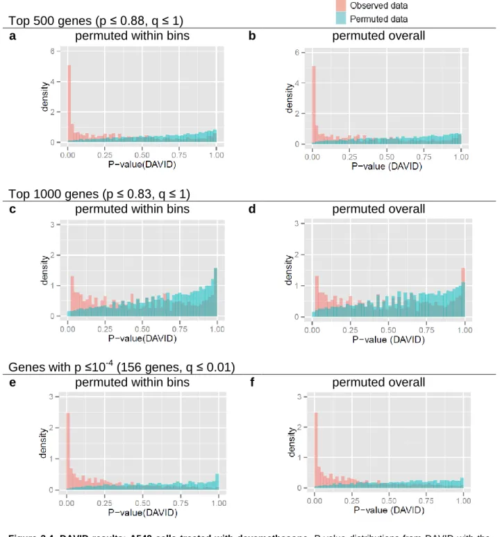
two different p-value to average read count trends ... 65 Figure 3.2. RNA-Enrich and random sets performance on permutated data ... 66 Figure 3.3. DAVID results: Prostate cancer LNCaP cells treated with an androgen
hormone.. ... 67 Figure 3.4. DAVID results: A549 cells treated with dexamethasone. ... 68 Figure 3.5. RNA-Enrich vs GOseq: Prostate cancer LNCaP cells treated with an
androgen hormone.. ... 70 Figure 3.6. Comparison of RNA-Enrich and Random Sets using DESeq2 differential
gene expression significance values ... 71 Figure 3.7. Comparison of RNA-Enrich and Random Sets using corrected fold change
as significance values. ... 72 Figure 3.8. RNA-Enrich vs random sets in tunicamycin-treated mouse embryonic
fibroblasts dataset using edgeR ... 73 Figure 3.9. RNA-Enrich vs random sets in tunicamycin-treated mouse embryonic
fibroblasts dataset using DEseq2 ... 74 Figure 3.10. RNA-Enrich vs random sets in tunicamycin-treated mouse embryonic
xi
Figure 4.1. Illustration of locus definitions and example of mappability calculation ... 96 Figure 4.2. Density curves of mappability of TSS extended loci show increased
mappability as read length increases. ... 97 Figure 4.3. Distribution of mappability and repetitive elements across different loci ... 98 Figure 4.4. Mappability of a Alu and L1 elements are positively correlated with age as
measured by percent divergence from consensus sequence ... 99 Figure 4.5. Scatterplots of mappability using 50mer reads and proportion of loci that are
Alu elements, L1 elements, and other repetitive elements show generally that gene loci that contain larger proportion of a repetitive element have lower
mappability and vice versa ... 101 Figure 4.6. Contribution scores of repetitive elements and segmental duplications are
correlated with mappability ... 102 Figure 4.7. Individual contribution of repetitive elements and segmental duplications to
mappability ... 103 Figure 4.8. Relationship of (a) mappability, (b) Alu elements, (c) L1 elements, and (d)
segmental duplications with gene length ... 104 Figure 4.9. Heatmap showing signed –log10(p-values) (negative for depleted terms,
positive for enriched terms) of GO gene set enrichment results ... 105 Figure 4.10. Mappability and locus length in human have similarly enriched gene sets.
Each point represents a GO term ... 106 Figure 4.11. Human and mouse have similarly enriched gene sets for (a) high and low
mappability and (b) long and short locus lengths. ... 107 Figure 4.12. NRSF ChIP-seq results ... 108
Supplementary Figures
Supplementary Figure 2.1. Gene loci with high (or low) average mappability are
enriched for specific Gene Ontology terms. ... 42 Supplementary Figure 2.2. Using the mappable locus length (locus length x mappability)
tends to improve the fit of the binomial cubic smoothing spline in the model, illustrated here with PAX5. ... 43
xii
Supplementary Figure 2.3. SIX5, PAX5, and H3K27me3 have different gene locus-length-to-peak presence relationships. ... 44 Supplementary Figure 2.4. The binomial test tends to identify gene sets with short locus length as significant (p < 0.05), especially for SIX5. ... 46 Supplementary Figure 2.5. The GREAT website test tends to detect gene sets with
shorter than average locus length, especially for SIX5. ... 47 Supplementary Figure 2.6. For SIX5 the ranks of the binomial test results from the
original data are highly correlated the average ranks from 25 permutations (within locus length bins) of the original data (Spearman r = 0.71). ... 48 Supplementary Figure 2.7. Relationship in simulated datasets between locus length and
presence of at least one peak (a-c), and QQ-plots showing the type 1 error rate of Fisher’s exact test, the binomial test, and ChIP-Enrich under these
relationships (d-f). ... 49 Supplementary Figure 2.8. Increasing overdispersion in peak counts among genes
increases the type 1 error rate of the binomial test, decreases type 1 error for Fisher’s exact test, and has no effect on ChIP-Enrich. ... 50 Supplementary Figure 2.9. Gene set enrichment testing using ≤ 1kb from TSS and
nearest TSS locus definitions often identifies very different sets of significant GO terms for the same DBP. ... 51 Supplementary Figure 2.10. A comparison of ChIP-Enrich GO term enrichment results
xiii
List of Tables
TablesTable 2.1 Comparison of top ranked GO terms for three DBPs from cell line GM12878 using ChIP-Enrich, FET, and the binomial test. ... 39 Table 2.2. Fisher’s exact test and the binomial test, but not ChIP-Enrich, show strongly
inflated type I error rates. ... 40 Table 2.3. Most significant Gene Ontology terms from GRα ChIP-Enrich analysis using
nearest TSS and ≤1kb from TSS locus definitions show a large degree of overlap with significant GO terms from RNA-seq data from the same cell line. ... 41 Table 3.1. Top ranked GO terms from RNA-Enrich for LNCaP cell line treated with DHT.
... 76 Table 4.1. Select significantly enriched/depleted GO terms. ... 109
Supplementary Tables
Supplementary Table 2.1. List of DBPs from Figure 2.1 with their total peak counts and associated peak caller. ... 53 Supplementary Table 2.2. Significant overdispersion in peak count among genes is
observed for a substantial number of GO terms in all 63 ENCODE ChIP-seq datasets from cell line GM12878 ... 55 Supplementary Table 2.3. GO terms most strongly associated with short locus length. 56 Supplementary Table 2.4. GO terms most strongly associated with long locus length. 56 Supplementary Table 2.5a. Top enriched GO terms (not collapsed, with ≤500 genes) for GR ChIP-seq data (4,392 peaks) that were significantly enriched (q ≤0.05) using the nearest TSS locus definition. ... 57 Supplementary Table 3.1. Extended version of Table 3.1. ... 76
xiv
Supplementary Table 4.1. Enriched and depleted GO terms for Alu and L1 elements, and segmental duplications for all locus regions (extended version of Table 4.1). ... 112 Supplementary Table 4.2. Full list of GO terms associated with clusters from Figure 4.9.
... 112 Supplementary Table 4.3. GO term enrichment results for mappability and locus length, comparing mouse and human. ... 112
xv
List of Abbreviations
Defined Abbreviations
cFC: corrected fold change 65
DBP: DNA binding protein 13
DE: differential expression 61
DEG: differentially expressed gene 5
DEX: dexamethasone 19
DHT: dihydrotestosterone 63
EtOH: ethanol 19
FAIRE-seq: Formaldehyde-Assisted Isolation of Regulatory Elements 3
FDR: false discovery rate 21
FET: Fisher's exact test 5
GO: Gene Ontology 5
GREAT: Genomic Regions Enrichment of Annotations Tool 12
GRα: glucocorticoid receptor α 13
GSE: Gene set enrichment 4
GSEA: Gene Set Enrichment Analysis 6
GWAS: genome-wide association studies 12
H3K27me3: trimethylation of histone 3 lysine 27 22
HTS: high-throughput sequencing 1
KEGG: Kyoto Encyclopedia of Genes and Genomes 5
L1: LINE-1 81
LINEs: long interspersed nuclear elements 80
LTRs: long terminal repeats 80
MEME: Multiple EM for Motif Elicitation 86
NRSF: neuron-restrictive silencer factor 86
PAX5: paired box 5 22
xvi
RPKM: reads per kilobase per million tags sequenced 19
SINEs: short interspersed nuclear elements 80
SIX5: SIX homeobox 5 22
TES: transcription end site 13
xvii
Abstract
Functional interpretation of high-throughput sequencing (HTS) data provides insight into biological systems, including important pathways in the context under study. A common approach is gene set enrichment (GSE) testing. GSE emerged in the age of microarrays as a way to biologically interpret long lists of differentially expressed genes (DEGs). However, HTS data has characteristics not present in microarray data that can bias GSE results. My thesis is focused on identifying, characterizing, and accounting for biases to improve functional interpretation in HTS data.
In this thesis, I present GSE tests designed for ChIP-seq data and RNA-seq data. Our tests have applications beyond HTS data, which we show by using them to analyze genomic features, including mappability and repeat content. ChIP-Enrich is a GSE test for ChIP-seq data. It includes a database of locus definitions to annotate peaks to different gene loci (such as exons, introns, promoters, and other intergenic regions), which allows for biological discovery unique to different regions. ChIP-Enrich empirically adjusts for the observed bias due to the varying lengths of these gene loci in its enrichment test. RNA-Enrich is a GSE test for RNA-seq data. RNA-Enrich corrects for the selection bias often observed in RNA-seq data, where long and highly expressed genes are more likely to be identified as DEGs. Unlike other GSE tests for RNA-seq data, RNA-Enrich does not require permutations or a cut-off to define DEGs, and works well with small sample sizes. For both ChIP-Enrich and RNA-Enrich, we showed well-calibrated type I error compared to competing methods. Finally, we characterize
sequence mappability, which is one potential bias in the interpretation of HTS data. We characterize properties of the main contributors of low mappability (transposons and segmental duplications), overall mappability, and their relationship with gene locus length and function. Across different transcribed and regulatory regions, certain gene functions showed unique signatures involving significantly more/fewer associated
xviii
repeats, higher/lower mappability, and longer/shorter locus length. Our analyses provide insight into evolutionary selection pressures that maintain complexity of gene regulation. Overall, we demonstrate that considering characteristics of the human genome is
1
Introduction
Chapter 1
1.1 Introduction
The era of high-throughput sequencing (HTS), also known as next-generation sequencing or massively parallel sequencing, has inspired progress in genomics that has produced an incredible amount of data. Along with generating the data, researchers have also developed various algorithms for each step of data processing. What starts as a multitude of short DNA sequences eventually undergoes quality control, genome alignment, gene assignment or quantitation, a myriad of statistical analyses, and then, finally, interpretation [1, 2]. Since the assembly of the human genome, we have
expanded high-throughput sequencing from sequencing of full genomes to a wide variety of applications that can measure gene expression [3], gene regulation and epigenetic marks [4]. The human genome is complicated but not random. Studying it poses many challenges. The organization of the human genome (e.g. exon/intron structures, spatial organization, and sequence redundancy) [5, 6] can perpetuate as biases in downstream analyses of HTS studies, resulting in incorrect interpretations of results, and therefore also may lead researchers to draw erroneous conclusions. This dissertation is focused on identifying, characterizing, and accounting for such biases to improve functional interpretation in various HTS platforms, including RNA-seq and ChIP-seq. Biases due to gene length, sequencing selection, and sequence mappability (the ability to uniquely align short DNA sequences) will be explored. While the research only includes select sequencing platforms, the findings and the methodology may be applicable to many types of current and, perhaps, future iterations of high-throughput sequencing technologies.
2
1.2 Background
1.2.1 High-throughput technologies
In this section, I explore some basic designs of popular high-throughput technologies, and pros and cons of each technology as relevant to this dissertation, beginning with the technology that predates HTS: microarrays. Prior to HTS,
microarrays were the tools of choice for measuring gene expression, copy number variation, DNA-binding (ChIP-chips), SNP genotyping, and more. They still remain popular in some areas of study such as DNA methylation and SNP genotyping. Gene expression microarrays make use of oligo hybridization and fluorescent labelling of probes to measure gene expression. Probes contain DNA sequence targets that are spread across the genome to target various parts of the gene body and/or intergenic regions. Probes occupy a small chip, and each sample cDNA (generated from sample RNA) can be PCR amplified to determine levels of expression based on the fluorescent signal. The Human MethylationEPIC BeadChip, for example, is the latest methylation microarray from Illumina and has over 850,000 probes that measure methylation using bisulfite-converted DNA across the genome. Many statistical applications for high-throughput data already existed for microarrays when next-generation sequencing was developed. Naively, approaches developed for microarrays were applied to sequencing data with little regard to whether underlying assumptions were correct. As I will further discuss in this dissertation, understanding the differences in data from microarrays and from sequencing is essential in developing the right tools, and for biological
interpretation.
The incentive to complete the Human Genome Project inspired next-generation sequencing technologies, which in turn motivated the development of a variety of molecular methods to explore a wide range of biological phenomena. The basis of massively parallel sequencing requires library preparation from select fragmentation of DNA. Fragments are then ligated to common adaptor sequences, and optionally
undergo multiple rounds of amplification to increase product input [7]. In RNA-seq, cDNA libraries can be prepared from RNA with specific features, for example those with a poly-A tail, a unique feature to mRNA [3]. Variations on RNA-seq to increase power to
3
detect specific isoforms and increase coverage include creating libraries that are paired-end and/or strand-specific. RNA-seq achieves a much higher dynamic range than
microarrays and is not subjected to the same selection bias that may occur due to probe placement. However, RNA-seq is not without its problems. Longer genes and more highly expressed genes are more likely to have more reads, and therefore are more likely to be called as significantly differentially expressed for many of the commonly used tests [8, 9]. In addition, sequenced fragments exhibit positional and sequence-specific preferences [10]. Several methods have been proposed to correct for such biases at the gene level [11-13], however if left uncorrected (or corrected for poorly), these biases can affect interpretation at the gene function level, e.g. gene set
enrichment testing – a topic I explore in Chapter 3 of this dissertation.
While RNA-seq is the HTS equivalent to gene expression microarrays, ChIP-seq is the HTS equivalent of ChIP-chip. ChIP is chromatin immunoprecipitation, a procedure to study the interaction between proteins and DNA in vivo. ChIP-chip is ChIP combined with microarrays, whereas ChIP-seq is ChIP combined with massively parallel
sequencing. In ChIP-seq, which is used to study genome-wide protein-DNA interactions (e.g. to identify transcription factor binding sites), libraries can be prepared from DNA bound by protein using an anti-body to target the particular protein of interest after crosslinking of protein and DNA, and then sample fragmentation. ChIP-seq has various modifications for applications beyond transcription factors. Histone modification ChIP-seq involves using antibodies that can detect specific histone tail modifications such as methylation or acetylation of one of the histone amino acids in the tetramer nucleosome protein complex. DNase-seq bypasses the antibody and performs fragmentation by targeting DNase hypersensitive sites with DNaseI digestion. FAIRE-seq (Formaldehyde-Assisted Isolation of Regulatory Elements) does not use antibodies and therefore is not limited to particular DNA-binding proteins. Proteins are crosslinked, followed by sample fragmentation, sonication, and then phenol-chloroform extraction of DNA [4, 14]. Similar to RNA-seq, ChIP-seq also has a selection bias, in that longer genes and genes with more intergenic space around them are often more likely to have an associated peak. Technically speaking, peaks are areas of the genome where there is a significant number of consensus sequence read alignments; biologically speaking, they are the
4
predicted protein-DNA binding sites. A study of the performance of a dozen popularly used peak calling algorithms [15] (including MACS, spp, and PeakSeq – three peak callers that have been used by the ENCODE consortium [16]) on ChIP-seq datasets for three transcription factors with different binding profiles, showed that the number of peaks identified can vary by tens of thousands among different peak callers. There are several newer peak callers [17-19] that have shown significant improvement in calling peaks with higher specificity – i.e. tested datasets produce peaks with high occurrence of binding motif and can be reproduced with ChIP and PCR. Unfortunately, it is often difficult to convince users to diverge from their usual protocol. Conceivably, a list of ChIP peaks that contains a substantial amount of false negatives may affect
downstream analysis if certain categories of genes consistently have many peaks or few peaks.
A critical step to analysis of HTS data is alignment of reads. Longer read lengths are more likely to uniquely align to areas of the genome but shorter reads may align to multiple places, and therefore are often less mappable (i.e. have less unique
sequence). Repeats pose a problem to sequence alignment. An estimated 45% of the human genome consists of repetitive elements called transposons [20, 21]. As we show in Chapter 4, they especially have a high occurrence in introns and intergenic regions. Alu elements, a type of short interspersed nuclear element, make up about 11% of the human genome and often occur near the transcription start site (TSS) [22]. Depending on how non-uniquely mappable reads are handled by the chosen sequence aligner, ChIP-seq peaks that occur near the TSS may be less likely to be detected if the peak region is not highly mappable. This also applies to any other region in the genome that is not uniquely mappable.
1.2.2 Gene set enrichment testing
Gene set enrichment (GSE) testing, also known as functional analysis of genes, is a way to identify important gene functions that differ between two different biological states. We have used it, for different genomic features like mappabiilty, repeat content, and gene length (Chapter 4). GSE can give insights into how a biological system works, and perhaps which pathways are important targets. GSE emerged in the age of
5
expressed genes (DEGs). Microarrays conquered the problem of obtaining gene expression profiles; however often the result was a list of hundreds or thousands of DEGs, which was simply too much information to absorb one gene at a time. The most common goal of GSE testing is to find pathways or biological processes that were affected by the conditions of an experiment. For example, in a microarray experiment that tested changes in gene expression before and after a drug treatment, GSE testing can enlighten researchers about which pathways were most affected by the treatment. In ChIP-seq data, one may be interested in discovering what biological processes are regulated by a transcription factor, or in what diseases it may play a role.
Gene sets may be constructed with various purposes in mind. Gene Ontology (GO), a commonly used gene set database, describes gene products in terms of biological processes, molecular functions, and cellular components [23]. The Kyoto Encyclopedia of Genes and Genomes (KEGG) pathways is a collection of manually drawn pathway maps representing molecular interactions and reaction networks [24]. Genes can also be classified into diseases (using MeSH terms or OMIM), spatially by open or condensed chromatin (cytoband), drug target lists, and many more. Typically GSE tests for overrepresentation, or enrichment, of gene sets. If the GSE test is two-sided, it may also test for underrepresentation, or depletion.
Several popular GSE methods exist for microarray data that are commonly applied to HTS data, three of which I will highlight here: Fisher’s exact test, GSEA, and random sets. Fisher’s exact test (FET) is a statistical test that analyzes contingency tables. In the case of GSE, the table is typically 2-by-2, where rows are gene set status (if the gene is in the gene set or not), and columns are gene significance status (for example, either differentially expressed or not, have a ChIP peak or not, etc). DAVID is perhaps the most widely used FET-based GSE test [25, 26]. DAVID modifies the FET by subtracting 1 from the table cell with the number of DEGs that are in the gene set. This modified FET is more conservative, it reduces the unpredictability of small gene sets, while having minimal effect on larger gene sets. Many implementations of FET exist besides DAVID, including GoMiner [27, 28] and HOMER [29] – which is designed for HTS data, allowing for association of peaks to genes as well as GSE testing. The underlying assumption of FET that is often violated with HTS data is that all genes are
6
assumed to have equal power (similar type II error rate) and to be equally likely to be a false positive (similar type I error rate). As we show in chapters 2-4, there are several factors that make a gene more or less likely to be identified as differentially expressed, have a peak, or any differential status.
Another widely used GSE method is GSEA, abbreviated from “Gene Set Enrichment Analysis”. GSEA uses a weighted Kolmogorov-Smirnov test, a
non-parametric test (i.e. it does not rely on a statistical distribution) [30, 31]. Input for GSEA is a ranked list of gene-level statistics, (for example, fold change ranked from most up-regulated to most down-up-regulated). A running-sum of the ordered gene-level statistics of genes in the gene set is calculated and compared to those not in the gene set to obtain an enrichment score. To calculate an associated p-value, a null distribution is generated by permuting phenotype labels, and the original enrichment score is compared to the distribution of permuted enrichment scores. There are several versions of GSEA that have been adapted for HTS data, including GSAASeqSP [32], which permutes read counts of genes, and SeqGSEA [33], which permutes the negative binomial statistics after using DESeq to test for differential gene expression. While GSEA, and some GSEA-like methods give the user the option to permute genes instead of phenotype labels, the GSEA authors recommend doing the latter, which “preserves gene-gene correlations and, thus, provides a more biologically reasonable assessment of
significance than would be obtained by permuting genes” [31]. However, this cannot be done with small sample sized experiments, because a sufficient number of unique permutations is required to obtain p-values with reasonable accuracy. Both
GSAASeqSP and SeqGSEA recommend sample sizes of at least 6-7 in each
phenotype for accurate GSE results. Often in HTS experiments, it is not feasible to have this many samples in each condition.
Finally, I would like to describe the random sets method for GSE testing [34]. Random sets is, in a way, a hybrid of FET and GSEA. While FET is limited to a binary gene status, the random sets approach, like GSEA, allows gene level statistics to be any general quantitative expression score, sg, for gene g. However, the test may not
behave properly if the distribution of scores, sg, is far from normally distributed. The
7
number of genes in gene set C. Intuitively, the enrichment score of one gene set is compared to random sets of the same size m that are drawn from the population of G genes (𝑚𝐺), however this comparison is done with a simple theoretical formula rather than performed directly, resulting in a quick, reproducible result. This approach is equivalent to permuting gene-level statistics among the gene labels. In the case where 𝑠𝑔 is binary, random sets reduces to FET. Newton et al (2007) showed the distribution of 𝑋̅ is approximately normal, and used the method of moments to determine a test
statistic and associated p-value for enrichment. While random sets does not require a binary gene status like FET, nor is it limited by small sample sizes like GSEA, it does continue to make the assumption that all genes are equally likely to be detected as significant (i.e. all genes have approximately the same power and same type 1 error). I expand on the performance of random sets in more detail in Chapter 3.
Other GSE tests mentioned in this dissertation belong to the class of model-based methods. LRpath, also developed for microarray data, uses a logistic regression model to test whether differential expression p-values, or any significance values of choice, for genes in a gene set are more or less significant than those for other genes [35, 36]. LRpath makes the same assumption that all genes are assumed to have equal power and equally likely to be a false positive. In Chapter 4, we use a different logistic regression GSE method, Broad-Enrich [37], that uses coverage proportion of gene (appropriate for HTS data like ChIP-seq of histone modifications) as the values of interest and corrects for gene locus length. In some cases, FET, GSEA, random sets, and LRpath can be applied to HTS data. However, as I will explain in this dissertation, the underlying assumptions of these tests are often not met with HTS data.
1.3 Overview of dissertation
Why is it important to account for bias in gene set enrichment testing? What are the origins of bias in HTS data? And what can we do to correct for these biases so that our conclusions are biologically sound? These are important questions that I seek to answer in this dissertation. Functional interpretation (e.g. GSE testing) bridges the gap between unwieldy, often hard to organize, high-throughput sequencing data and
8
identification and characterization of the biases in the current state of HTS technology. It is important to note both technical and biological biases, as sometimes both are not mutually exclusive and often will affect the accuracy of conclusions that one draws from analyzing HTS data.
In Chapter 2, we present a gene set enrichment test, called ChIP-Enrich, that was designed for ChIP-seq data and other assays that produce a list of relatively narrow genomic regions (peaks). To perform GSE testing with ChIP-seq data, peaks have to be assigned to genes. The common practice is to assign peaks (defined by their midpoints) to the nearest TSS. As I have mentioned before, genes with longer loci are more likely to have a peak assigned to them. We address the bias of gene locus length in
assignment of ChIP-seq peaks to genes, and developed a method that empirically adjusts for the observed bias. In doing so, we created a database of locus definitions to annotate peaks to different loci, such as introns, exons, nearest TSS, and 5kb around a TSS, therefore requiring different locus length adjustments and allowing for biological discovery that may be unique to different regulatory regions. We demonstrated that ChIP-Enrich is able to correct for all kinds of peak-to-locus-length relationships while maintaining a good type I error. We also introduce the significance of correcting for sequence mappability, which I expound upon in Chapter 4. In the ChIP-Enrich project, my contributions as a co-first author, in addition to helping to write the manuscript, were: (1) creating the locus definitions for the available genomes; (2) calculating mappability values for different kmer lengths and genomes; (3) applying ChIP-Enrich to 63 different ENCODE ChIP-seq datasets; (4) along with co-first author Ryan Welch, performing permutation testing on select ENCODE datasets to show how type I error rates of ChIP-Enrich compared to competing methods; (5) analyzing and interpreting a case study on a glucocorticoid receptor ChIP-seq dataset from ENCODE in respect to its regulatory activity in promoter and distal regions; and (6) assisting in creating the R Bioconductor package, chipenrich and chipenrich.data that are also employed on our website:
http://chip-enrich.med.umich.edu/.
In Chapter 3, we present a gene set enrichment test, RNA-Enrich, to address a selection bias often observed in RNA-seq data where long and highly expressed genes are more likely to be identified as significantly differentially expressed (i.e. not all genes
9
have the same power). We modify the random sets method to adjust for average read count per gene. To calculate a test statistic for gene set enrichment, we determine a weight based on the observed relationship between read count and significance values in the data. In datasets where there is no relationship, RNA-Enrich approximates random sets. In datasets where there is a relationship, correcting for the bias allows for improved identification of truly enriched or depleted gene sets. We compare RNA-Enrich to other GSE methods: random sets, DAVID, GOseq, GSAASeqSP and SeqGSEA. We also implement RNA-Enrich using significance values from different sources, including differential gene expression p-values from two different methods and a corrected fold change instead of p-values. We show that using average gene read count as a proxy for the selection bias greatly improves the type I error compared to other GSE tests for RNA-seq data.
Chapter 4 delves into sequence mappability, its relationship with repeat elements and gene length, and their correlation with gene function. We perform GSE testing using highly prevalent transposons in the human genome: L1 elements, which are a type of long intersperse nuclear element, and Alu elements, a type of short intersperse nuclear element. Together, these two repetitive elements make up an estimated 26% of the human genome. Segmental duplications, which are long duplications of DNA sequence that are 1-200kb in length and have >90% identity, make up 5% of the human genome. We show that across different regulatory regions, certain gene functions show unique enrichment signatures of Alu elements, L1 elements, segmental duplication,
mappability, and gene length. That is, certain types of genes have significantly
more/fewer associated repeat elements, higher/lower mappability, and longer/shorter gene locus length. While sequence mappability is a technical measurement that depends on sequence read length, we show that it can elucidate genomic architecture that relates to gene length and repeat elements. Our analyses gives insight into how evolutionary selection has been used to maintain the required complexity of gene regulations, and which types of genes have been most affected.
10
ChIP-Enrich: Gene set enrichment testing for ChIP-seq
Chapter 2
data
2.1 Introduction
Genome-wide high-throughput experiments can assess transcription factor binding, epigenetic marks, differential gene expression or disease association, and often result in thousands of identified genomic regions or genes. Gene set enrichment testing is one way to determine how these lists of genomic regions or genes are related biologically, e.g. by assessment of Gene Ontology (GO)) terms [38-40]. For ChIP-seq experiments, oftentimes thousands of transcription factor binding sites or histone modification sites are identified. Enrichment testing of this data, or with a union or intersection of multiple ChIP-seq datasets, can identify key biological processes, functions, disease gene signatures, or other biological concepts regulated by the factor(s) under the given experimental conditions [41]. Conversely, ChIP-seq data can be used to create gene sets against which other experimental datasets can be tested for significant enrichment, including other ChIP-seq data [42, 43].
Gene set enrichment tests can generally be classified as competitive [36, 39, 44], self-contained [31], or a hybrid [31, 45], as discussed by Efron and Tibshirani in [46]. The hypothesis of competitive approaches is that there is a higher proportion of
identified genes (or a higher level of significance overall) in the gene set of interest than in the remaining genes. In contrast, self-contained methods only use information about the genes in the gene set of interest, and test whether the significance level of the set is greater than expected given a null hypothesis. The enrichment testing methods used for sets of genomic regions (ChIP-seq data), including FET and binomial based tests, are
Chapter 2 is published as Welch RP*, Lee C*, Imbriano PM, Patil S, Weymouth TE, Smith RA, Scott LJ, Sartor MA: ChIP-Enrich: gene set enrichment testing for ChIP-seq data. Nucleic Acids Research 2014, 42(13).
11 all competitive approaches [40, 47].
Fisher’s exact test (FET), and slight variations on it, have traditionally been used for gene set enrichment in microarray gene expression data [39, 48-51]. FET makes the assumption that each gene has an equal probability of being identified as significant. Across gene sets, this means that each gene set is expected under the null hypothesis to have approximately the same proportion of significant genes as the overall proportion of significant genes. In contrast to microarray data, the data generated from ChIP-seq, RNA-Seq, and genome-wide association studies (GWAS), often show a positive
correlation between the length of the relevant genomic region and detection of the gene [9, 52, 53]. In ChIP-seq data, the probability of a peak occurring within a gene or its surrounding non-coding sequence, which together we denote as the gene locus, is often positively correlated with the length of the locus [54]. Due to this correlation, genes with longer locus lengths contribute a disproportionate amount to the enrichment signal, and this bias introduced in the signal due to gene locus length violates the assumptions of FET. Furthermore, because many commonly tested gene sets contain genes with substantially longer (e.g., developmentally and nervous system related genes) or shorter (e.g., electron transport, rRNA processing) than average locus length [54], the gene sets with longer or shorter than average locus length are more or less likely, respectively to be detected as significantly enriched [53]. Therefore, lack of effective adjustment for gene locus length can lead to false positive findings.
Several approaches have been developed to adjust for locus length in ChIP-seq [47], RNA-Seq (for example, GOseq) [9], and GWAS data [52, 55]. For ChIP-seq data, a commonly used binomial-based test asks if the total number of peaks within the loci in a gene set is greater than expected, given the total locus length of the gene set, the total number of peaks and the corresponding length of the genome (implemented in
Genomic Regions Enrichment of Annotations Tool (GREAT)) [47, 53]. In contrast to FET, the assumptions of the binomial test are met when the number of peaks in a locus is proportional to locus length, and the variability of peak counts among genes, given gene locus length, is consistent with that expected by the binomial distribution.
We examined the gene locus length-to-peak presence relationships in 63 ENCODE ChIP-seq GM12878 datasets and found they ranged from no relationship to
12
strongly positively correlated. Given these observations, our goal was to develop a gene set enrichment method for ChIP-seq data (ChIP-Enrich) that empirically models and adjusts for the relationship between locus length and peak presence. ChIP-Enrich maintained the expected type I error rate (false positive rate) in all tested datasets, whereas FET and the binomial test did not. For each DNA binding protein (DBP), we asked if different (potential) regulatory region definitions would identify different
enriched/disenriched gene sets. For the glucocorticoid receptor α (GRα), we examined the ability of ChIP-Enrich to detect known and potentially novel functions. Our method is freely available in the R Bioconductor package chipenrich and as a web-based program (http://chip-enrich.med.umich.edu).
2.2 Materials and Methods
2.2.1 Experimental ChIP-seq peak datasets
We used ENCODE ChIP-seq peak datasets from 63 DNA binding proteins for cell line GM12878 [56] (see http://chip-enrich.med.umich.edu/SummaryEncode.jsp)
(Supplementary Table 2.1). We used the existing peak calls, which were called by the original authors using one or two of three peak calling methods (MACS, spp or Scripture [57-59]). For the subset of datasets that were called by two callers (MACS and spp), we use results from MACS, as we generally observed a larger number of called peaks for MACS than for spp.
2.2.2 Gene loci definitions and presence of peaks in a locus
We define a gene as the region between the furthest upstream transcription start site (TSS) and furthest downstream transcription end site (TES) for that gene. The positions of the TSSs and TESs for each gene were extracted from the UCSC knownGene table (human genome build hg19). We removed small nuclear RNAs as they are likely to have different regulatory mechanisms than other genes and often reside within the boundaries of other genes. For gene set enrichment testing we assign ChIP-seq peaks to genes (based on the peak midpoint) using three primary definitions of a gene's designated regulatory region (locus definitions). 1) Nearest TSS: the region between the upstream and downstream midpoints between a gene and the two
13
adjacent genes' TSSs. This is equivalent to assigning each peak to the gene with the nearest TSS. 2) Nearest gene: the region from the midpoint between the TSS and the adjacent gene's TSS or TSE (whichever is closest) to the midpoint between the TES and the adjacent gene’s TSS or TES (whichever is closest). This is equivalent to assigning peaks to the nearest gene. 3) ≤1kb from TSS: the region within 1kb of all TSSs in a gene. If TSSs from the adjacent gene(s) are less than 2kb away, we use the midpoint between the two TSSs as the boundary of the locus for each gene. Additionally we define ≤5kb from TSS, using the same rules as we defined ≤1kb from TSS, and we define >10kb from TSS, by subtracting the 10kb regions around the TSS from the nearest TSS locus definition. We define peak presence in a locus as ≥ 1 peak midpoint within the gene locus boundaries.
2.2.3 Gene Ontology terms
GO terms from GO molecular functions, GO cellular components, and GO biological processes were extracted from Bioconductor species specific annotation packages and the GO.db R package. We removed genes from each GO term that do not exist in our gene locus definitions as these genes could not have a peak assigned to them. For testing in the manuscript and in our tool, we exclude GO terms with <10 genes as they have more limited power to detect significant results, and as a rule of thumb logistic regression requires at least 10 events for each explaining variable [60]. In the manuscript, we also exclude reporting GO terms with >500 genes, as the categories become broader and less informative in interpreting the results. Q-values were
calculated using all GO terms with 10-2000 genes (our tool’s defaults).
2.2.4 Overdispersion test of peak count (given locus length) in each gene set
Overdispersion is defined as higher variability in a data set than expected based on the distribution used to model it. The binomial test in GREAT uses a binomial
distribution to model the combined number of peaks for all genes in a gene set, so if significant overdispersion in peak counts exists among genes, the binomial distribution assumption is not satisfied. We tested for overdispersion in the number of peaks per gene (given locus length) in each gene set using Tarone’s Z statistic [61]. Tarone’s Z
14
allows better estimates of overdispersion when the binomial probabilities are close to 0 or 1 (the probabilities of having a peak for each basepair are very close to 0). We tested all gene sets with a minimum of 50 genes (as gene sets with fewer genes often do not have adequate power for this test) and a maximum of 500 genes (the maximum gene set size used throughout the paper). For each DBP, we reported the proportion of gene sets that had significantly higher variability than expected based on the binomial
distribution (q-value≤0.05).
2.2.5 Mappability calculations
To estimate the mappable proportion of each gene locus for different read
lengths, we first calculated base pair mappability for reads of lengths 24, 36, 40, 50, 75, and 100 base pairs using mappability data for Homo sapiens (build hg19) from the UCSC Genome Browser. The UCSC browser mappability tracks provide, for each base pair i, the reciprocal of the number of locations in the genome to which a read beginning at i and extending for read length K could map; a value of 1 indicates the read maps to one location in the genome, a smaller value indicates the read maps to two or more locations in the genome. We set reads with mappability <1 to 0 and calculated base pair mappability as the average read mappability of all possible reads of size K that include a specific base pair location, i,:
𝐵𝑖 = ( 1
2𝐾 − 1) ∑ 𝑀𝑗
𝑖+(𝐾−1)
𝑗=𝑖−𝐾+1
(equation 1) where Bi is the mappability of base pair i, and Mj is the read mappability (from UCSC’s
mappability track) of a read of length K beginning at position j. We define gene locus mappability, m, as theaverage of all base pair mappability, Bi, values for a gene locus;
each gene locus mappability score m represents the proportion of the gene locus that is uniquely mappable (given the read length of the data).
2.2.6 ChIP-Enrich method
We developed a logistic regression approach to test for gene set enrichment while adjusting for log10 mappable locus length for each gene. Suppose that for a given
set of genomic regions (referred to as peaks), we have assigned each peak to a gene locus. The dependent variable is a binary vector defined as 1 if ≥1 peak is assigned to a
15
gene’s locus, and 0 if none are assigned to the gene’s locus. For each gene set, the explanatory variable of interest is gene set membership, g, defined as 1 for genes in the gene set, and 0 for all other genes. Let L be the locus length, such that m∙L is the
mappable locus length. Let be the probability that a gene with gene set membership g, and adjusted for mappable locus length, has ≥1 peak. Then
1
are thecorresponding odds that a gene, given g = 0 or 1 and mappable locus length m∙L, has ≥1 peak. If the log-odds differ by gene set membership adjusted for (mappable) locus length, then we conclude that peak presence is associated with the gene set. Our model is:
log 1
1 log 0 1 10 g f mL (equation 2) where 0 is the intercept, 1 is the coefficient of interest, and the function f(log10(m∙L+1)) is a binomial cubic smoothing spline term that adjusts for log10 mappable locus
length (or log10 locus length if m is omitted). We apply the log10 transformation to locus
length as this improves the model fit (data not shown). The smoothing spline is
estimated with a penalized spline using a cubic spline basis fit with 10 knots distributed evenly throughout the data. Placing a knot at each data point as in a true smoothing spline would not be computationally feasible. The model is fit using penalized likelihood maximization, where the smoothing penalty is the squared second derivative penalty, and generalized cross-validation is used to choose the optimal value for the smoothing parameter, [62, 63]. We use the gam function of the R package mgcv to fit the model [64], and the Wald statistic to test for significance of the gene set term, β1,which is
calculated as: 2 1 ˆ 1 ˆ s W (equation 3)
where ˆ1 is the penalized maximum likelihood estimate for , and sβˆ1 is the standard
error forˆ1. W is distributed as 2
with one degree of freedom under the null hypothesis β1=0, and p-values are calculated accordingly for the alternative hypothesis, β1≠0. P-values for the gene sets are corrected for multiple testing using the Benjamini-Hochberg false discovery rate approach [65]. To be included in the analysis, genes had to be
16
annotated in GO and have a locus defined. For example, we have 19,051 human genes with the nearest TSS locus definition and 16,653 (87.4%) of these genes have ≥ 1 GO term annotation (with no restriction for GO term size).
2.2.7 R package and website
Our ChIP-Enrich gene set enrichment testing method is implemented in the chipenrich package for the R statistical software environment and available through Bioconductor, and as a web version at http://chip-enrich.med.umich.edu/. We also provide Fisher’s exact test as an alternative enrichment method. In addition to Gene Ontology, we include 12 additional annotation sources containing over 20,000 total gene sets [35]. We currently support the human genome (hg19), mouse genome (mm9, mm10), and rat genome (rn4). Precomputed mappability is available for hg19 (for read lengths specified above) and for mm9 (read lengths 36, 40, 50, 75, and 100 base pairs). Users may either supply an R data frame (for the R package) or a BED format file
containing the peak locations as input. Runtime is typically 10-14 minutes for testing all GO terms but varies depending on the dataset, number of cores, and choice of locus definition. In addition to the nearest TSS, nearest gene, ≤1kb from TSS and ≤5kb from TSS locus definitions, described above, in ChIP-Enrich we also offer Exons: peaks are assigned to gene exons, ignoring all peaks outside of an exon. Users may also supply their own custom locus definition and/or mappability file. This enables users to study functional binding patterns relative to alternative gene features (e.g., 3’UTRs) or at different distances from TSSs, and to use different estimates of the observable region for each gene locus. Diagnostic plots are available to visualize the relationship between locus length and proportion of genes with a peak, and to examine the proportion of peaks binding proximal or distal to TSSs. We also offer an ENCODE ChIP-Enrich Results website (http://chip-enrich.med.umich.edu/summaryReport.jsp ), where users can download enrichment testing results for individual DBPs or in bulk for the GM12878 and K562 cell lines.
17
2.2.8 Fisher’s exact test for gene set enrichment testing of ChIP-seq data
For each GO term, we tested for association of peak presence and GO term membership using a two-sided Fisher’s exact test. For inclusion in the analysis, genes had to be annotated in GO and have a locus defined.
2.2.9 Binomial test for GO term enrichment testing of ChIP-seq data
We used a slight modification of the one-sided binomial test for GO term
enrichment described by Taher et al (2009) [53] and implemented in GREAT [47]. We calculate the one-sided probability of seeing greater than or equal to the number of peaks we observe for a GO term, π, with the following formula:
∑𝑛𝑖=𝑘𝜋(𝑛𝑖 ) 𝑝𝜋𝑖(1 − 𝑝𝜋)𝑛−𝑖 (equation 4)
where n is the total number of peaks within gene loci present in any GO term, and kπ is
the number of peaks annotated to GO term π. We define pπ as the expected proportion
of peaks in GO term π, as the total non-gapped length of the gene loci in the GO term, divided by the total non-gapped length of loci with ≥1 GO term annotation. P-values are calculated as the probability of observing kπ or greater number of peaks in the GO term.
Our implementation is consistent with other GO term enrichment programs which restrict the background gene set to those annotated in GO [66]. In contrast, GREAT uses the total non-gapped genome as the denominator for pπ and defines n as all
observed peaks.
2.2.10 Permutations to create ENCODE ChIP-Seq data with no biological enrichment
We performed permutations to assess the behavior of each enrichment test under two null scenarios of no true enrichment. For both scenarios, we used three ENCODE ChIP-seq datasets from cell line GM12878: SIX5 (Figure 2.1a,d), PAX5 (Figure 2.1b,e), and H3K27me3 (Figure 2.1c,f). For each of the two permutation
scenarios below, we perform 300 permutations and test each permuted dataset for GO term enrichment (5519 GO terms) using the three tests (ChIP-Enrich, Fisher’s exact test, and the binomial test).
18
Under both scenarios, we do not expect to detect enrichment, as we have removed any association between gene membership in GO terms, and the count of peaks. To help visualize the two permutation scenarios, consider a data table, where each row represents a gene, and contains the following columns: count of peaks per gene, locus length of each gene, and one column for each GO term containing a (0,1) indicator variable for whether the gene belongs to that GO term. In the GO term
permutations scenario, we randomly permute the count of peaks per gene and the locus length as a unit. This results in a dataset where genes (identified by their peak count and locus length) have been reassigned to new GO terms and the locus length bias inherent in GO terms has been removed, but the number of genes per GO term,
correlations between GO terms, and the relationship between locus length and count of peaks have all been preserved. In the GO term permutation by locus length bin
scenario, we first order the data by locus length and then randomly permute peak count and locus length as a unit, but restrict this permutation within successive bins of gene locus length (100 genes per bin). This is similar to the first scenario, but preserves the relationship between locus length and GO term membership.
2.2.11 GRα analysis
We applied ChIP-Enrich to ChIP-seq peaks for GRα data from the A549 cell line from Reddy et al (2009): ChIP-Seq peaks with FDR <0.02 (4,392 peaks). In Reddy et al (2009), sequence reads of 36mer length, were generated from Illumina GA1, aligned using ELAND, and peaks were called using MACS. Reddy et al. (2009) identified 209 genes as differentially expressed based on RNA-Seq data from A549 cells that were treated for 1hr with 100mM of Dexamethasone (DEX) or with 0.02% Ethanol control (EtOH). Briefly, in Reddy et al. (2009), gene expression levels were estimated using ERANGE to calculate reads per kilobase per million tags sequenced (RPKM) values, which were then adjusted for dependence of variance on expression level. A custom maximum likelihood approach was used to calculate p-values for the observed change in gene expression between DEX-treated and ethanol-treated cells. Finally, genes with FDR<0.05 were called significant [67]. Using the 209 reported differentially expressed genes, we tested for GO term enrichment (over-representation) with the R package goseq [9]. For Table 3, we pruned the list of top-ranked, enriched GO terms of closely
19
related terms for presentation by removing terms whose parents, children, or siblings in the ontology tree were present at a higher rank in the list. We used the R package GO.db to determine relationships among GO terms.
2.3 Results
2.3.1 Observed relationship between gene locus length and presence of at least one peak in ENCODE ChIP-seq datasets
We first explore the relationship between gene locus length and the presence of a peak in 63 ENCODE ChIP-seq datasets from tier 1 cell line GM12878 [16, 56] using a binomial cubic smoothing spline to model the relationship (see Experimental ChIP-seq peak datasets and ChIP-seq method sections of Methods) [62, 63]. GM12878 is a lymphoblastoid cell line, transformed using Epstein-Barr Virus, and which has a normal karyotype. Lymphoblasts are immature cells that typically differentiate into lymphocytes, and serve as a good model for functional studies as they are known to express a wide range of metabolic pathways [68]. This exploration of ChIP-seq data is motivated by the opposing assumptions underlying FET and the binomial test: for FET that there is no association between locus length and presence of a peak, and for binomial-based tests, that the number of peaks per locus is proportional to locus length. In Figure 2.1, we assigned peaks to the gene with the nearest TSS (see Methods) and grouped the ENCODE datasets based on the total number of peaks (three equal sized groups). For datasets with the smallest number of peaks, we noticed that a large fraction of peaks were close to a TSS, and there was no or little relationship between locus length and probability of a peak (Figure 2.1a,d; n=21) which is consistent with the assumptions of FET. All were transcription factor datasets. In contrast, datasets with the largest number of peaks tended to have the smallest proportion of peaks within 1kb of a TSS and had a strong positive locus length-to-peak presence relationship (Figure 2.1,f; n=21), which is potentially consistent with the assumptions of the binomial test. Many of these datasets were histone modifications that tend to occur much more widely across the genome than TF binding. The locus length-to-peak presence patterns within datasets with
20
intermediate numbers of peaks show larger variability and are often not consistent with either FET or the binomial test assumptions (Figure 2.1b,e).
The binomial test sums the peaks over all the genes/loci in a gene set. This summation assumes that the underlying probability of a peak per unit length is the same for each gene in the gene set (and the same for each gene not in the gene set), i.e. the variance of peak counts among genes in a gene set is no greater than expected based on the binomial distribution. We tested for variability greater than that of the binomial distribution, in GO terms containing between 50 and 500 genes. All DBPs showed a substantial proportion of GO terms with significantly (FDR<0.05) higher variability than expected, with many DBPs having over 99% of GO terms with significant extra
variability (Supplementary Table 2.2) (see Overdispersion test in Methods). Thus, even DBPs that have a strong positive relationship between number of peaks and locus length (Figure 2.1f) do not satisfy the binomial test assumptions.
2.3.2 ChIP-Enrich method
Given the observed locus length-to-peak presence relationships, we sought to develop a gene set enrichment testing approach for ChIP-seq data that would
empirically model this relationship (Figure 2.2). To capture different aspects of the underlying regulatory biology, we define loci based on one or more genomic features, and assign peaks in the defined genomic regions to genes (locus definitions). In this paper we use as primary locus definitions: 1) the region(s) within 1kb of every TSS of a gene (≤1kb from TSS), 2) the region between the upstream and downstream midpoints between a gene’s TSS and the adjacent genes' TSSs (nearest TSS), and 3) the gene and half the intergenic region between adjacent genes, defined by the closest TSS/TES of each gene (nearest gene) (See Gene loci definitions section of Methods for more details). Consistent with previous observations [54], genes with long locus lengths defined by the nearest TSS definition were significantly enriched for neuronal
processes, development, and adhesion (Supplementary Table 2.3), while genes with short locus lengths were enriched for translation and chromatin-related processes (Supplementary Table 2.4),
We test for gene set enrichment using a logistic regression model, and adjust for the probability of a peak as a function of log10(observable locus length) using a
21
binomial cubic smoothing spline (see ChIP-Enrich method section of Methods). Since a logistic regression model without the smoothing spline term approximately corresponds to Fisher’s exact test, our model is motivated by FET while accounting for locus length. Because we observed that the average mappability of gene loci both differed
substantially among genes and that many GO terms were enriched with highly or lowly mappable genes (Supplementary Text and Supplementary Figure 2.1), we also account for the average mappability of each gene locus. We calculate the proportion of each locus length that is uniquely mappable as the mappability score, and use locus length × mappability as an estimate of the observable locus length (see Mappability Methods section). Although mappability often improved the spline fit (Supplementary Figure 2.2), it had little effect on the results of these analyses. Our R package and web-based tool offer a number of additional options, including custom locus and mappability definitions (see R package and website Methods section). Thirteen gene annotation databases [35] are available for testing; for simplicity, we use GO terms to illustrate our method in our analyses below (see Gene Ontology terms Methods section).
2.3.3 Comparison of ChIP-Enrich, Fisher’s exact test and the binomial test for permuted and non-permuted ENCODE datasets
To illustrate the performance of the different tests, we selected three ENCODE GM12878 DBPs with different locus length-to-peak presence relationships: SIX homeobox 5 (SIX5) (weak relationship, Figure 2.1d), paired box 5 (PAX5) (moderate positive relationship, Figure 2.1e), and trimethylation of histone 3 lysine 27 (H3K27me3) (strong positive relationship, Figure 2.1f) (Supplementary Figure 2.3). These DBPs have 75, 26, and 5% of peaks ≤1kb from a TSS (Figure 2.1a-c) and 4,442, 19,618 and
41,464 total peaks, respectively. We first tested for GO term enrichment with FET, the binomial test, and ChIP-Enrich in the original data (see Methods for implementation details of FET and the binomial test). The top ranked terms from the three tests were highly different for H3K27me3, moderately different for PAX5, and similar for SIX5 where several very strongly enriched GO terms were identified by all tests (Table 2.1 Comparison of top ranked GO terms for three DBPs from cell line GM12878 using ChIP-Enrich, FET, and the binomial test.). However, other datasets with total peaks
22
counts similar to SIX5 (few peaks) (Figure 2.1a,d) had less agreement between the top ranked terms for ChIP-Enrich and the binomial test (data not shown).
Under the null hypothesis of no true gene set enrichment, the type I error rate for a dataset at a given threshold α is the proportion of gene sets with p-value less than α. A method with type I error rate higher than the expected α level will have an increased number of false positives. Therefore, we investigated the type I error rates for ChIP-Enrich, the binomial test, and FET. We assessed the type I error rate using two
permutation scenarios that preserve the GO term correlation structure but under which no biological enrichment exists, and therefore none should be detected. In the first scenario, we grouped gene locus length and gene peak count and permuted them together across all genes, which removes any relationship between GO term
membership and locus length (permutations across all genes). In the second scenario, we grouped locus length and gene peak count and permuted them together within bins of 100 genes ordered by locus length, which retains the GO term-locus length
relationship (permutations within locus length bins) (see Permutations Methods section). In the permutations across all genes, ChIP-Enrich and FET showed slightly conservative type I error for both permutation scenarios at α=0.05 and 0.001 (Table 2.2 and Supplementary text), with the slight deflation expected due to the discrete nature of the data [69]. The lack of inflation for FET was expected since this permutation breaks the GO term-locus length relationship. In contrast, the binomial test had very high type I error rates at all three tested alpha levels (Table 2.2).
For the permutations within locus length bins, ChIP-Enrich again had the expected type I error rate (Table 2.2). FET showed inflation of type I error rates for PAX5 and H3K27me3, but not for SIX5. SIX5 shows little relationship between locus length and peak presence, and therefore the assumptions for FET are approximately satisfied. As a check of the ChIP-Enrich method, we compared the –log10(p-values) in the original SIX5 data and found they were highly correlated between ChIP-Enrich and FET (Pearson’s r=0.97), illustrating that in this case ChIP-Enrich closely approximates Fisher’s exact test. The binomial test again had very high type I error rates for every DBP, with particularly high error for H3k27me3 (minimum permuted p-value = 1 × 10-57). Using the binomial test we observed 761 gene sets with p<0.001 in the original