11 ii
THE ECONOMIC
AND SOCIAL
RE SEARCH INSTITUTE
MEMORANDUM SERIES
139
k
A Note on OLS MultNar|ate Regress|on w|th Suggest|ons for
AddiHons to Routine Computer Programmes
R. C. Geary
k
Confidential: Not to be quoted
until the permission of the~ Author
(i)
o
Let the OLS regression be:-k
Y=a+i-)=~b’X’+e’l 1
Geary h.as argued, somewhat controvertially, that the individual coefficients
b. are meaningful only in the cases of simple regression or of each pair of the
1
k indvars X. being not significantly correlated, very rare in practice. Then,
1
and ouly then, could one state "a rise of 1 in X. causes a rise of b. in Y."
Other-1 1
wise this inference is false. The argument holds that the only valid purpose of
the multiple regression is the estimation of Y, usually in the form of extrapol~ion
of time series beyond the esti,nation period. This memos that the coefficient
vector ~a, b1, b2, c!ements.
... bk~ is objectively memlingful, but not its individual
There is not much point in extrapolation of time series ".unless the ~2 is near unity and the DW or tau are near their white noise values, i.e. near
2 and near half the number of residues respectively. On account of the usu,-d
high h~tercorrelation when the indvars are time series, most researchers prefer
to work with the deltas, ~ Y and AXi, a procedurewhich incidentally will usually
considerably reduce and in some cases eliminate intercorrelation between the
indvars, i.e. the pairs of X. may be highly correlated but not the pairs o~X..
1 1
DW owes its inception entirely to assessment of residual autocorrelation
in the case of time series, and this because of a characteristic property of time
series, namely that they are au,~ocorrelated to start with. The thoughtprocess
is as follows. Y, to be explained, is a time vector. Treating it as an OLS residual
(i.e. fitting merely a eonstml~ to it) we compute its DW as -T
1)2 2 =
---(2) DW= +S=’2 (Y’~- Yt- / ~g-yt’ Yt Yt- Y’
,and customarily find that this DW has .’: very low value, well below 2, iadic~lli~\q
-2-OLS regression but there would be no point in using DWor tau as indicating
completeness of re!ationship, since all the DWs and tans would be near their
white noise values, i.e. likethe original Ys the successive values of the residuals
would be random to one another. Or, given original time series data, Y, X1,X2, ...,
Xk, randomizing these would make no difference in computation to the values of
the coefficients but it would destroy the useful role of DW or tau, the values of
which depend on the ordering of the data.
Reverting then to the typical time series case of Y’s having a very
low value of DW, we imagine ourselves computing the OLS regressions successively
Y on one X (simple regressions}, on two Xs ete and computing DW or tau on the
residuals in each case. We stop when we have found a DW or tau which indicates
that the residuals are probably random to one another. There may be several
such sets because of intercorrelation between the X’s. There are computer
programmes for systematic selection of the best sequence of Xs to bring into
the GLS regression, so avoiding an immense series of such regressions.
With time series when, with one’s OLS regression, one has obtained
-2
an R near 1 and DW or tau indicating probable residual randomness (or white
noise), one may go ahead with e.xtrapolation in time, such extrapolated estimates
being subject to known probabilistic ranges of error. One may be wrong, perhaps
due to new variables {i. e., other than the Xi) affecting the relationship, but one
may at least state that as far as past experience goes the extrapolations should
be as stated.
The multiple regression computer prints-out have the silly habits
of producing DWs, even when time series are no.~.t involved. Such values are
meaningless, a remark which would apply also to the tau value. To repeat, the
essence of time series is that time automatically orders the data (Y, Xi) in a
particular way. In the non-time series case (say cross-section) the data should
one indvar, say X1) the obvious course would be to reorder the residuals according
to the magnitude of X1 and then compute DW or tau; if Y or X1 are related this
will result in Y being ordered, generally increasing or decreasing, i.e. autoregressed
like time series. In the case of multiple regression the best course might be
to reorder the residuals according to the magnitude of the princiPal compone’nt
of the indvars. Could not the computer be programmed to do this ?
At one time I thought that this problem of indvar intercorrelation
could be bypassed so as to make the coefficients meaningful by substituting for
the matrix of indvars the matrix of components. These are linear functions of
the original variables Xi and number also k, and have the precious property that
each pair is exactly uncorrelated (i.e. for each (i, j) j ~ i r.. = 0). This procedure Ij
might have the added beaus of reducing the number of indvars, i.e. only the
first one, two or three having statistically significant coefficients.
The trouble about using their principal components instead of
original indvars is that the latter have identity and the former have not. Thus,
if one were studying the effect of a change in social weffare payments or,
unemployment, one indvar might’be B.M. Walsh’s percentage of s.w. payments
to wages together with other indvars, the depvar the unemployment rate. Suppose
thatthe coefficient of the ratio X1 was significant, its value b1. It would be
perfectly sensible to ask "What would be the effect on Y of an increase of 1
in X1 7", even if the answer were not b1. But if the first component were, say,
t, t
XI and its significant coefficicint bl, it would simply be meaningless to ask what
t
would be the effect on the unemployment rate of an ~.crease of 1 in Xi, because,
! ,
tn general, we donTt know what X1 is; we cantt describe it. The same remark
applies to other components with even greater force since, while the principal
component ia a sense synthesizes all the !ndvars, the other components are much
-4-To some minds the statistically significant individual coefficients
can be regarded as having a meaning because of the Frisch-Waugh theorem which
states that the b1 is exactly the value which would be found from a simple regression
-(3) RY =aI+blRX1 ÷eI,
R being a symbol for residue, in fact the residues when Y and XI are each OLS
-regressed on the remaining indvars (X2X3 ... Xk). So it would be right to state
that bI is the effect of a change of 1 in the first variable on the depvar when each
of those two variables have been corrected for the effects of the other indvars.
the form
-Oeary generalized Frisch- Waugh to the following effect. Write (1) in
.!k k! + k2 (4) Y =a÷1=’~ lbl.Xl+ ~:bjXj.+e
j = k1 + 1
with k1
k1 and k2.
+ k2 = k, the variables having been divided arbitrarily into two groups Of
Then
-k,
(5) RY =a1+.~ bIRX. +eI,
I=l l
the Rs indicating the residues when the variables Y, X1," X2, ... Xkl, and each
OLS - regressed on Xkl+ 1’ "’" Xk1 + k2" The bi in (4) and (5) would be identical.
This would have been an efficient way to calculate the coefficients of (1) using
a primitive calculating machine but has little practical point with the advent of
the computer, apart from algebraic interest, in providing a meaning for individual
regression coefficients.
I
The statement, based on the original regression, that a change
of 1 in X1 would result in a change of b1 in Y v;ould be valid were it not for. the
necessary condition which is that the other indvars remain unchanged. In general
the latter c ond[t[en is unacceptable because if there is a significant correlation
between X1 and any other variable, say X2, X2 Cannot be presumed to remain
The previous paragraph hints at a procedure which might yield an
answer to the question of the effect on the depvar of an increase of 1 ih a particular
lndvar, say X1. Regress all the other indvars on X1
-(6) Xl=al+bilXi, 1=2, 3, ..., k.
One infers that a rise of 1 in X1 would entail a rise of bil in X.. Hence the total
effect of a rise of 1 in X1 will be found by substituting the Values 1, b21, b31, ...
bkl for the k indvars in (1), ignoring e.
All praetitloners agree that it is a sound principle in multiple regression
-2 to use as few indvars as possible consistent, of course, with high values of R
and residual randomness. This may be the place to remark that the s~tistical
process of OLS regression Is anything but an exact science. Wise judgment is
¯ of the essence, such jtldgment being based on a plentiful supply of computer data
derived from ample routine computering. One must be very careful about
elimination of indvars.
One’s original set of in’dvars are presumably those which theory or
simple ratiocination indicates might be related to the depvar and whose (depvar,
lndvar) simple correlation is statistically significant. But here it might be
argued that it might be prudent to retain the variable in one’s set even if
ul,correlated with the depvar, since with otherindvars it may be correlated.
Anyway, assume that one has a large set of indvars to start with.
1~2 One begins with an OLS regression on this whole set. The" F or test
wll; Indicate Its significance. If insignificant there is no point in going ahead.
If DW or tau indicates residual autocorrelation new indvars should be sought.
If the 1~2 is close to unity on the original set of indvars the OLS regression may
be, useful for extrapolation even with "bad" DWs and tans, on the assumption
-6-that some of the variables have insignificant values, Leave these out and repeat
the OLS regression. If this emission does not alter the value of ~2 much the omission
is justified: the trouble here is (and where judgment enters) is that we have no
way of knowing how much is "much". If the value of ~t2 is lowered one must experiment
further as to which of the low-coefficient indvars to retain in the set. One must
not automatically reduce one’s original set of indvars because onwhole-set regression
their coefficients are insignificantly small, Leser-Geary have shown that one can
have significant OLS regression (by the F test) with all coefficients not significant
In a multiple regression; it is only in simple regression (one indvar) that the F
and t (eo~ficient) tests are absolutely consistent with one another, as regards
probabilistic inference. Multivariate regression is the OLS regression process
of the depvar on the whole set of indvars in which It Is impossible to isolate
Individual lndvars. In this sense all regression is "simple".
It is suggested that the following be added to routine computer
processes for OLS regression
-(1) In non-time OLS regression, reorder residuals according to magnitude of
principal component of indvars (or of the magnitude of the single indvar
In the case of simple regression) before calculation of DW or tau,
(Ii) for assessing the effect of an increase of 1 in each indvar on the depvar,
allow for the effect of all other indvars by according the variable in question,
say Xi, the value 1 and other variables the value bji given by the simple OLS regression
(7) Xj =aj+bjiXi+ej ~j~i.
The print-out would give the values of b.. and the actual values on the depvar of
jt
an Increase of 1 for each indvar.
)
The computer can select the "best" set of indvars from a large Initial
set when It is given the rules of selection. In this and other application the computer
application, for instance, all pairs of c.e. s in (Y, Xi) should be given, perhaps the bji Suggested here as well¯
A weakness in the bji proposal is that (7) (and indeed all OLS regressions)
Is a cause-effect statement, in (7) X. is the cause of X.. This may not be the
l j
ease. A statement neutral to cause - effect might be better. "a rise of 1 m X.
1
tl
will be accompanied by a rise of c.. in X.. This issue of cause-effect v. functional
J, J
was much discussed years ago and techniques evolved for dealing with the neutral
ease. These techniques are difficult, indecisive and generally unsatisfactory,
so OLS procedure may remain if as a p[s aller¯
Significance in OLS regression is nearly always assessed by reference
to a null-hypothesis table for the F test using degrees of freedom: with number
of sets of data T and number of indvars k, these are k (numerator) and (T - k -1)
(denominator). One is confronted with the problem of deciding by F which of a
set of regressions based on different sets selected from the large original set
Is the best. Now the present computer programmes of which I am aware simply
yield the value of F. It would be better that the NHP should be given¯ It is
admitted that this would be much to expect since it implies the store’s containing
al..l the null-hypothesis frequency distributions of F for tw...~o dimensions of degrees
of frequency. The F table I use has simply the critical NH values of F for each
pair of d.f. and a number of two.ended probability levels, the lowest. 005: for
Instance, with d.f.s 7 (= k) and 24 (i.e. number of sets of observations is 32 = T),
:,:~’ = 3.99. One assesses that NHP is less than. 005 if one. obtains a value
of F greater than 3.99 but one does not know what this probability is.
Now the regression is not much use unless the actual value of F does not
greatly exceed the lowest NHP tabled value. It also happens that the tabled NHP
values vary greatly with the number of indvars k. Thus for probabilities. 005
and. 05 and T = 32~
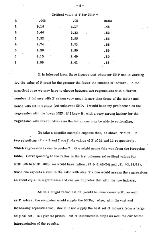
¯ ¯ m 8 k .005 1 9.18 2 6.40 3 5.32 4 4.74 5 4.38 6 4.15 7 3.99
Critical value of F for NHP =
.05 Ratio 4.17 .45 3.33 .52 2.95 .55 2.73 .58 2.59 .59 2.49 .60 2.42 .61
It is inferred from these figures that whatever NHP one is working
to, the value of F must be the greater the fewer the number of indvars. In the
practical case we may have to choose between two regressions with different
number of indvars with F values very much larger than those of the tables and
hence with infinitesimal (but unknown) NHP. I would base my preference on the
regress!on with the lower NHP, if I knew it, with a very strong hanker for the
regression with fewer indvars as the better one may be able to rationalize.
To take a Specific example suppose that, as above, T = 32. In
°
two selections of k = 2 and 7 one finds values of F of 24 and 13 respectively.
C
[image:9.576.31.551.17.828.2]Which regression is one to prefer ? One might argue this way from the foregoing
table. Corresponding to the ratios in the last columns (of critical values for
NHP. 05 to NHP . 005) we would have ratios . 27 (= 6.40/24) and . 31 (=3.99/13).
"d
Since one expects a rise in the ratio with size of k one would assess the regressions
as about equal in significance and one would prefer that with the two indvars.
All this turgid ratiocination would be tmneccessary if, as well
as F values, the computer would supply the NHPs. Also, with its vast and
increasing sophistication, should it not supply the best set of indvars from a large
original set. But give us prints - out of intermediate steps as well for our better
°
interpretation of the results.
Would ESI~I computer experts interest themselves in devising a
programme ineorporatlug the points in this note ?
As a short footnote to the foregoing assessment of - the aggregate
effect of a rise of 1 in X. on y, it might be asked "Should not insignificantly valued l
bjis be omitted (i.e. regarded a having value zero)?"I have no strong views on the
subject and would value those of my colleagues. I am inclined to favour leaving
all values in because of (i) simplicity for the computer, (Hi) the values may be
genuine (e. g. "sign right" according to theory), (iii) values will be small and with
different signs, so that effect of inclusion or exclusion on answer to "increase
of 1" will lie within the confidence limits of the latter.
18 January1980 R.C. Geary.