warwick.ac.uk/lib-publications
Original citation:
Crevillén-García, D. (2018) Surrogate modelling for the prediction of spatial fields based on
simultaneous dimensionality reduction of high-dimensional input/output spaces. Royal
Society Open Science, 5 (4). 171933. doi:10.1098/rsos.171933
Permanent WRAP URL:
http://wrap.warwick.ac.uk/102722
Copyright and reuse:
The Warwick Research Archive Portal (WRAP) makes this work of researchers of the
University of Warwick available open access under the following conditions.
This article is made available under the Creative Commons Attribution 4.0 International
license (CC BY 4.0) and may be reused according to the conditions of the license. For more
details see:
http://creativecommons.org/licenses/by/4.0/
A note on versions:
The version presented in WRAP is the published version, or, version of record, and may be
cited as it appears here.
rsos.royalsocietypublishing.org
Research
Cite this article:Crevillén-García D. 2018
Surrogate modelling for the prediction of spatial fields based on simultaneous dimensionality reduction of high-dimensional input/output spaces.R. Soc. open sci.5: 171933. http://dx.doi.org/10.1098/rsos.171933
Received: 16 November 2017 Accepted: 20 March 2018
Subject Category:
Mathematics
Subject Areas:
applied mathematics/computer modelling and simulation
Keywords:
stochastic PDE, simultaneous dimensionality reduction, Gaussian process regression, spatial field emulation
Author for correspondence:
D. Crevillén-García
e-mail:[email protected]
Surrogate modelling for the
prediction of spatial fields
based on simultaneous
dimensionality reduction of
high-dimensional
input/output spaces
D. Crevillén-García
School of Engineering, University of Warwick, Coventry CV4 7AL, UK
DC-G,0000-0001-5981-7961
Time-consuming numerical simulators for solving groundwater flow and dissolution models of physico-chemical processes in deep aquifers normally require some of the model inputs to be defined in high-dimensional spaces in order to return realistic results. Sometimes, the outputs of interest are spatial fields leading to high-dimensional output spaces. Although Gaussian process emulation has been satisfactorily used for computing faithful and inexpensive approximations of complex simulators, these have been mostly applied to problems defined in low-dimensional input spaces. In this paper, we propose a method for simultaneously reducing the dimensionality of very high-dimensional input and output spaces in Gaussian process emulators for stochastic partial differential equation models while retaining the qualitative features of the original models. This allows us to build a surrogate model for the prediction of spatial fields in such time-consuming simulators. We apply the methodology to a model of convection and dissolution processes occurring during carbon capture and storage.
1. Introduction
The use of complex mathematical models for simulating and predicting the behaviour of physico-chemical processes is nowadays crucial in a broad range of groundwater disciplines, including contaminant transport and geological storage of CO2
in deep saline aquifers among many others. The complexity of these models normally involves the implementation of highly demanding and time-consuming numerical codes, and thus there
2
rsos
.ro
yalsociet
ypublishing
.or
g
R.
Soc
.open
sc
i.
5
:1
71933
...
is growing interest in designing faster and reliable statistical approximations of the computationally expensive simulators, so-called emulators.
The vast majority of physico-chemical processes in porous media can be successfully described using stochastic partial differential equations (SPDEs) (see [1–5]). One parameter of special relevance in these equations is the permeability of the porous medium used to describe the inherent random heterogeneity of the rock formation. Several researchers have shown in the past that although permeability values can exhibit large spatial variations, these variations are not entirely random but spatially correlated (e.g. [1–3]). It has been also shown through experimental validation that permeability fields can be successfully modelled using a log-Gaussian distribution assumption (e.g. [4]). For instance, Maraet al.
[6] modelled strongly heterogeneous aquifers by using a stochastic Gaussian process (GP) for the log-transmissivity fields conditional on data sampled at a set of locations in an aquifer. One of the most extended possibilities to generate samples of a log-Gaussian random field is through Karhunen–Lo´eve (KL) decompositions of the correlation function of the underlying Gaussian field evaluated at each of the grid points of the computational domain (see [5,7]). These samples are represented by a sequence of indexed random coefficients in a finite series. An immediate consequence of this form of representation of the input fields is that the dimension of the stochastic input space is as high as the number of grid points in the computational domain. As an example, for standard meshes of size 50×50, 80×80 or 100×100 in a two-dimensional rectangular domain, we would need to deal with a few thousands of stochastic degrees of freedom (DoF) if we do not wish field variance preservation to become an issue. In other words, the hypothetical over-smoothing of the generated permeability fields caused by a further truncation of the original KL decomposition, if not handled properly, would lead to unrealistic results.
During the past decade, several high-dimensional model representation (HDMR) techniques, e.g. CUT-HDMR, adaptive HDMR and new truncated HDMR, have been developed to reduce the high-dimensionality of stochastic input spaces (see [8–12]). HDMR methods split the original high-dimensional model into a set of lower-high-dimensional sub-models leading to less computational effort when solving the resulting sub-models by any numerical method. One of the preferred methods to be complemented with HDMR techniques for solving high-dimensional SPDEs found in the literature is the stochastic collocation (SC) method in any of its variants, e.g. full-tensor product, Smolyak sparse grid etc. (see [11,13–17]). The SC method became so popular because, besides providing fast convergence, it lies within the so-called non-intrusive methods for solving SPDEs, i.e. neither knowledge nor algebraic manipulation of the equations that will be solved is required, and thus researchers can use existing in-house or commercial numerical simulators to implement the method. However, for some groundwater models (e.g. [5,7,18]) the number of stochastic DoF needed for an acceptable resolution of the results is still prohibitive for this method. One of the alternatives to overcome the problem of high dimensionality in time-demanding groundwater model simulators is GP emulation [19–21].
There are several applications of GP emulation of multivariate simulators, for instance Bowmanet al.
[22] compared four different techniques for emulating multivariate outputs in atmospheric dispersion models. To the best of our knowledge, there are still a limited number of publications in the literature dealing with GP emulation of groundwater models in very high-dimensional input spaces (e.g. [5]). GP emulators for high-dimensional simulators also necessitate HDMR methods to overcome the limitations of Bayesian regression. These limitations frequently arise in the estimation of some of the model parameters (so-called hyperparameters) present in anisotropic covariance/correlation functions. The hyperparameters area prioriunknown and need to be estimated from the data provided by the simulator. The maximum-likelihood estimate (MLE) method has been extensively employed to find estimates of the hyperparameters (see [5,23,24]). Most of the optimization algorithms used to find the MLE (in our case by minimizing the negative log marginal likelihood), for instance steepest descent, conjugate gradient, Hessian-free Newton etc., are critically dependent on the selection of the initial guess to initialize the iterative algorithm. This sensitivity to the choice of the initial values might be, for instance, due to the existence of multiple local maxima in the marginal likelihood [21]. While these methods have been satisfactorily used to estimate hyperparameters defined in low-dimensional spaces, for high-dimensional spaces this has historically led to an optimization problem, and in most of the cases to complete failure. In groundwater models, GP emulators normally represent point correlation by using automatic relevance determination covariances [25], and for these cases, we propose a continuation algorithm for passing the right initial values to the MLE method in the successive iterations. This will overcome the optimization issue and will make feasible the MLE method for a moderate/high dimension of the input space.
3
rsos
.ro
yalsociet
ypublishing
.or
g
R.
Soc
.open
sc
i.
5
:1
71933
...
high-dimensional input and output spaces, and in particular for groundwater model simulators. Note that standardscalarGP emulation has already been successfully applied to complex and time-consuming scalar valued simulators [5]. Thus, the inputs and outputs of the simulator considered here will be spatial fields defined in very high-dimensional input and output spaces. The GP emulator is able to reproduce (up to a predetermined level of accuracy) the work of the computer model much faster. This is of vital importance in applications such as uncertainty quantification, design optimization and decision theory, where a large number (sometimes millions) of calls to the numerical simulator are required in order to produce a critical assessment. The methodology of the empirical simultaneous GP model reduction (ESGPMR) approach presented in this paper consists of combining two main techniques. (i) We use the method proposed by Higdonet al.[26] to reduce the dimensionality of the output space by using principal component analysis (PCA) and separate independent GP emulators for the coefficients in the PCA basis. Higdon’s approach has been successfully adapted to other applications, for example, Holden
et al.[27] applied a variation of the method to high-dimensional climate model outputs. Bowman & Woods [22] adapted the method to the field of atmospheric dispersion by using the thin-plate splines technique. (ii) We capture the high-dimensional relationship between the simulator inputs and the coefficients of each of the vectors spanning the reduced output space by exploiting the properties of the KL decomposition of the input permeability fields and using cross-validation (CV). Thus, we find a subspace of the high-dimensional input space leading to an optimal representation of the GP model response surface. To test the GP emulation results, we take as reference (true value) a sample of 256 full numerical simulations. The simulations were obtained over 18 days of continuous intensive CPU computations on a 12-core Intel Xeon cluster processor. The time spent to compute the final prediction of the same 256 spatial fields with the ESGPMR approach on the same processor was 4 h.
The outline of this paper is as follows. In §2, we introduce the computationally expensive numerical simulator of a convection and dissolution process in random heterogeneous porous media. In §3, we describe the framework of the GP emulation methodology. We present the novel method for simultaneous input–output model dimension reduction and we detail how to properly estimate the hyperparameters of a high-dimensional space by using a continuation algorithm. In §4, we test the GP model reduction methodologies with the model problem introduced earlier. Concluding remarks are provided in §5.
2. Mathematical model and numerical simulator
Dissolution of CO2in deep saline aquifers is considered one of the most effective ways of carbon capture
and storage [28]. The model studied here focusses on the hydrodynamical part of the problem by setting a model for CO2-loaded flows in an idealized two-dimensional geometry. It considers the impact of
hydrodynamic dispersion (or dispersivity), permeability heterogeneity and isotropy in porous media on the development of convecting instabilities. For solving the resulting problem, the finite-element method (FEM) is employed. The existence of continuous bifurcations from the no-flow steady-state solutions of the problem adds additional challenge to the search of numerical solutions, and to overcome this an arclength continuation technique [29] is used in conjunction with the FEM.
2.1. Convectively enhanced dissolution process in porous media
The dissolution of CO2into the brine of the storage site causes an increase in the density of the mixture,
leading the CO2 to sink while reacting with local rock minerals to become a solid carbonate [30]. This
leads to the onset of convection rolls and the resulting mixing leads to a greater contact between the injected CO2 and local minerals, significantly enhancing the carbon capture. This process is known as
convectively enhanced dissolution (C-ED) [31,32].
In recent theoretical and numerical works (e.g. [32–34]), researchers have investigated the behaviour of CO2in deep saline aquifers. These studies focussed on the understanding of a simplified and idealized
case where the problem is reduced to the motion of a fluid through a porous medium and where the dispersive transport is based on pure molecular diffusion. This paper will take into account more characteristics of natural aquifers, namely the rock heterogeneity and the hydrodynamic dispersion. This later will be modelled by a dispersion tensor,D, dependent on the local Darcy velocity of the fluiduas follows [34–36]:D=DmI+βTuI+(βL−βT)(u⊗u/u), where⊗represents the tensor product,Iis
the unit (identity) tensor,Dmis the molecular diffusion coefficient of the solute in the fluid andβLand βT are, respectively, the longitudinal and transverse dispersion coefficients, which satisfyβL≥βT≥0
4
rsos
.ro
yalsociet
ypublishing
.or
g
R.
Soc
.open
sc
i.
5
:1
71933
...
We consider the C-ED process to occur in a two-dimensional domain representing a random, heterogeneous, isotropic porous medium of depth 2Hand lengthL. The spatial variable is defined by
x=(x,z) on the domain [0,L]×[−H,H]. The governing equations for this model are continuity (2.1), Darcy’s Law (2.2) and convection–diffusion-reaction (2.3) [32,33,38]:
∇ ·u=0, (2.1)
u= −K
μ(∇P+ρgez) (2.2)
and φ∂∂C
t +u· ∇C=φ∇ ·(D∇C)−γcC, (2.3)
whereezis the outward-pointing unit vector along the ordinate axis,Cis the concentration of dissolved
CO2, u=(ux,uz) is the fluid velocity andP is the fluid pressure. The parameters K, μ, φ, γc and g
are, respectively, the medium permeability field, the fluid viscosity, the rock porosity, the reaction rate and acceleration due to gravity. The solute undergoes a first-order reaction and is converted into an inert product with no effect on the solution density, thus the density of the fluid is linearized and takes the form, ρ=ρ0+βcC, where ρ0 andβc are the density of the pure fluid and the volumetric
expansion coefficient. This assumption allows us to use the Boussinesq approximation [32]. The boundary conditions for the above problem are:C(x,z=H)=C0 andux(0,z)=ux(L,z)=uz(x,±H)=0,
(∂C/∂z)(x,−H)=(∂C/∂x)(0,z)=(∂C/∂x)(L,z)=0.
The velocity field is represented by using a streamfunction,Ψ, formulation, ux=∂Ψ/∂zanduz= −∂Ψ/∂x. We can eliminate the pressure field from equation ((2.2)) by satisfying the mass conservation (2.1), resulting in a new set of equations for the unknown field variables (Ψ,C). For the resulting set of governing equations and boundary conditions we follow the same dimensionless formulation used in Crevillén-Garcíaet al.[5], where the reader can find a full detailed derivation of formulae and equations. The dimensionless variables and numbers are defined by: x=x/H, z=z/H, Ψ=Ψ μ/HC0K0βcg,
C=C/C0, t=tC0K0βcρ/μφH, βL=βLC0K0βcg/D0μ, βT =βTC0K0βcg/D0μ, K=K/K0, L=L/H, Ra=
K0C0gβcH/φμD0 and Da=γcμH/K0C0gβc, where βT and βL are, respectively, the longitudinal and
transverse dispersion coefficients [37,38];K0andD0are reference permeability and diffusion coefficients,
respectively;Lis the aspect ratio of the domain;Rais the Rayleigh number, related to the buoyancy driven flow; andDa is the Damkhöler number, which is the ratio of the chemical reaction rate to the mass transfer rate [32]. In terms of these dimensionless variables and numbers, and dropping the primes for convenience, the following dimensionless governing equations defined inR=[0,L]×[−1, 1] stay as:
∂ ∂x
1
K
∂Ψ ∂x
+∂∂
z
1
K
∂Ψ ∂z
+∂∂C
x=0 (2.4)
and
∂C
∂t −
∂Ψ ∂z
∂C
∂x +
∂Ψ ∂x
∂C
∂z −
1
Ra
∂
Jx ∂x +
∂Jz ∂z
+DaC=0. (2.5)
The Fickian mass flux J=(Jx,Jz) (Scheidegger-Bear) [38] satisfies J=D∇C and its components
are expressed as follows: Jx=(1+βT∇Ψ2)(∂C/∂x)+((βL−βT)/∇Ψ2)((∂Ψ /∂z)2(∂C/∂x)−(∂Ψ /∂x)
(∂Ψ /∂z)(∂C/∂z)) and Jz=(1+βT∇Ψ2)(∂C/∂z)+((βL−βT)/∇Ψ2)((∂Ψ /∂x)2(∂C/∂z)−(∂Ψ /∂x)(∂Ψ / ∂z)(∂C/∂x)), where · 2denotes the standard Euclidean norm. Finally, the corresponding dimensionless
form of the boundary conditions is: C(x, 1)=1, Ψ(x,±1)=Ψ(0,z)=Ψ(L,z)=0, (∂C/∂z)(x,−1)= (∂C/∂x)(0,z)=(∂C/∂x)(L,z)=0. In this study, we are interested in the long-term behaviour of the system and consequently we will restrict ourselves to the steady-state equations, i.e. by setting∂C/∂t=0 in equation (2.5).
2.2. Convectively enhanced dissolution numerical simulator
5
rsos
.ro
yalsociet
ypublishing
.or
g
R.
Soc
.open
sc
i.
5
:1
71933
...
2.3. Generation of random permeability fields
Natural media is heterogeneous in a hierarchy of scales, and it is virtually impossible with today’s technologies to resolve this heterogeneity in detail [43]. The permeability values have shown spatial correlation [1–3] and a function that has been extensively used [2,5,7,18,44,45] to represent that correlation is the following squared exponential covariance function:
c(xi,xj)=σ2 exp
−x
i−xj2 λ
xi,xj∈R, (2.6)
whereλrepresents the correlation length andσ2the variance of the process.
The simulator described earlier necessitates the values of the permeabilityKat each of theMnodes of the computational domain in order to solve the problem. It is common in groundwater flow models [18] to modelKas a log-Gaussian random field; this guarantees thatK>0 inR. In this study, we will model the permeability as log-Gaussian permeability fields and generate samples of the permeability fields at the nodes with the following procedure [46]. Let (Ω,F,P) be a probability space. If we now let Z∼N(m,C), i.e. Z:Ω→RM be a multivariate normally distributed random vector with mean
and covariance m=(m1,. . .,mM)=E[Z]∈RM, C=E[(Z−m)(Z−m)]∈RM×M, respectively, where
mi=E[Z(xi)]=m(xi),Cij=c(xi,xj), i,j=1,. . .,M. Then, given the set of nodes{xi}Mi=1, the vectorZ:=
(Z(x1),. . .,Z(xM))is a discrete Gaussian random field. Finally, we setK=exp(Z) to obtain the desired discrete log-Gaussian permeability field, where each of the components of the vectorK∈RMcorresponds to the value of the permeability at a node of the computational domain.
To generate different samples ofZ, we will use the KL decomposition method (see [5,7,46,47]. This method uses an eigen-decomposition of the covariance matrixCat the nodes which is then stored for future samples generation. Moreover, the KL expansion may be truncated, which leads to a reduced-dimensional formulation that is critical in the emulator construction. The KL decomposition method is summarized as follows.
The covariance matrixCis real-valued and symmetric, and therefore admits an eigen-decomposition [48]:C=(ΦΛ1/2)(ΦΛ1/2), whereΛis theM×Mdiagonal matrix of ordered decreasing eigenvalues λ1≥λ2≥ · · · ≥λM≥0, andΦis theM×Mmatrix whose columnsφi,i=1,. . .,M, are the eigenvectors of
C. Letξi∼N(0, 1),i=1,. . .,M, be independent and identically distributed (i.i.d.) random variables. We
can draw samples fromZ∼N(m,C) using the KL decomposition ofZusing the following expression [46]:
Z=m+ΦΛ12(ξ1,. . .,ξM)=m+
M
i=1
λiφiξi. (2.7)
The termsξi∼N(0, 1) are calledKL coefficients. To be consistent with the non-dimensional formulation
of equations (2.4) and (2.5), we generate a set of log-Gaussian permeability fields with point-wise mean 1 by settingm= −(σ/2)I. Let us define the random vectorξ∈RM, distributed according toN(0,I). The
numerical simulator is considered as a mapping fromξ∈RMto (C,Ψ)∈RM×RM. If we were interested only in one of the two simulator output fields, we could also consider the simulator as eitherfc:ξ→C
orfΨ:ξ→Ψ.
In the next section, we will describe how to build a GP emulator.
3. Gaussian process emulation of spatial fields in complex simulators
6
rsos
.ro
yalsociet
ypublishing
.or
g
R.
Soc
.open
sc
i.
5
:1
71933
...
successive iterations. The continuation routine can be easily made extensive to any existing moderate-dimensional GP emulators that groundwater researchers using commercial GP toolboxes discarded because of the impossibility of estimating the hyperparameters appropriately. In the next section, we only give a brief description of the GP framework, stating our choices for the prior specifications of the GP model, the generation of the training data and the final predictive equations used to approximate the simulator. For a detailed description of conditional distributions and the derivation of the final formulae, we refer the reader to Rasmussen & Williams [21].
3.1. Gaussian process emulation framework
In this section, we describe the general GP emulation methodology for scalar functions, to then extend it to vector functions in the next section. Letg:RM→Rbe a scalar simulator. The aim of GP emulation
is to learn the functional form of the target modelg(·) in the light of a very reduced (due to the time-consuming simulator) set of data. The design points can be regarded as the locations (in the input space) at which we wish to obtain the values ofg(·) to determine the sensitivity of the simulator to different inputs. An exhaustive explanation of the possible choice of design points is addressed in Sackset al.[19]. To generate the set of design points, we simply spread the points to cover the input space, in this case
RM. There are several methods of sampling the inputs, the most common of which are Latin hypercube
sampling (LHS) [49,50] and Sobol sequence sampling [51]. In this paper, guided by the successful results obtained in a previous work, we will use the latter. Given the particular definition of the inputs in our model simulator (ξ∼N(0,I)), one very intuitive way of building a set ofddesign points is to, first, use a Sobol sequence to generatedpoints in [0, 1]M, and second, push thedpoints component-wise through the inverse cumulative distribution function ofMrandom variables distributed according toN(0,σd2), withσd2≥1, to, jointly, form the set of design pointsξˆj=(ξˆj1,. . .,ξˆjM), j=1,. . .,d. Note that by setting σd>1, we guarantee that the design points are spread enough inRM to cover all the points sampled
from the input distribution (N(0,I)), and therefore we will not be missing some key information about the simulator responses at points far from the mean of the input distribution.
Let us denote byf(·) the GP used to modelg(·). For anyξ,ξ∈RD, for someD≤M, the GP prior mean
function is defined as:m(ξ) :=E[f(ξ)] and the covariance function as:k(ξ,ξ) :=Cov(f(ξ),f(ξ))=E[(f(ξ)−
m(ξ))(f(ξ)−m(ξ))], where E[f(·)] and Cov(·,·) denote the expectation and covariance operators, respectively. One of the methods available in the literature to select the mean and covariance functions for a given model is CV (see [5]). However, the covariance chosen for this GP makes no difference to the scope of the approaches developed in this study, and thus, for simplicity, we will use a mean-zero function and the square exponential (SE) covariance which is given in terms of three hyperparameters as follows [21]:
k(ξ,ξ)=σf2exp(−21(ξ−ξ)diag(1−2,. . .,−D2)(ξ−ξ))+σn2δij, (3.1)
whereσf2 is the process variance,=(1,. . .,D) is the length scale,σn2 is the noise variance andδij is
the Kronecker delta. The hyperparameters are collectively represented byθθθ=(σf2,,σn2). Given the set of
design points generated with the method described earlier,ξˆj=(ξˆj1,. . .,ξˆjM),j=1,. . .,d, we can define
thedesign matrixas X=[ξˆ1,ξˆ2,. . .,ξˆd]. To avoid numerical instabilities (ill-conditioning of the matrix
system), an i.i.d. random noisej∼N(0,σn2), whereσn2is the variance in expression (3.1), is typically
introduced into the model, and thus the observed values will take the formyj=fc(ξˆj)+j, whereyjis the
perturbed simulator output at the design pointξˆj∈RM. If we now writey=[y1,. . .,yd], we can define
thetraining setas the pairD= {X, y}. Once we have provided the model with a mean-zero function, the SE covariance function (3.1) and the training setD, we can make predictions for new untested inputs
ξ∗∈RDby using the predictive equations for GP regression [21]:
mD(ξ∗)=Σ(ξ∗,X)[Σ(X,X)+σn2I]−1y (3.2)
and
kD(ξ∗,ξ∗)=k(ξ∗,ξ∗)−Σ(ξ∗,X)[Σ(X,X)+σn2I]−1Σ(ξ∗,X), (3.3)
where the (i,j)th entry of Σ(X,X)∈Rd×d is given by k(ξˆ
i,ξˆj) and Σ(ξ∗,X)=(k(ξ∗,ξˆ1),. . .,k(ξ∗,ξˆd)).
7
rsos
.ro
yalsociet
ypublishing
.or
g
R.
Soc
.open
sc
i.
5
:1
71933
...
3.2. Reduced-rank approximation of the output space
In this section, we use the method proposed by Higdonet al.[26]. The idea is to use PCA to project the original simulator outputs onto a lower-dimensional space spanned by an orthogonal basis. This is done via singular value decomposition (SVD) as we detail later. Once in the PCA framework, the outputs can be expressed as a linear combination of PCA basis vectors (or the principal components (PCs)) with coefficients treated as independent univariate GPs with distinct sets of correlation lengths. This allows us to build separate GP emulators (as many as PCs considered) to estimate the coefficients of new outputs at untested inputs in the PCA basis. Then we use a linear map for reconstruction to the original output space. By using orthogonal projection, we guarantees a minimal average reconstruction error. The error considered for comparisons between two vectors throughout this paper will be the L2-norm relative
error (RE) unless stated otherwise. For the two vectorsx=(x1,. . .,xM) andy=(y1,. . .,yM), we define
theL2-norm RE betweenxandyas
RE(x,y)=x−y2
x2 , (3.4)
wherex2is the Euclidean norm.
Let us consider a simulator (e.g.fc) which receives inputs inRMand returns outputs inRM(instead
of R). Then the GP emulator described in §3.1 would not work. Let Y be the M×d matrix with columnjthejth run of the simulator. The dimension reduction in the output space can be described as follows:
(i) Subtract off the mean for each dimensionMto obtain the centred version of the matrixY,Y. (ii) Multiply the centred matrixYby the normalization constant 1/√d−1 to obtainY.
(iii) Compute the SVD ofYand obtain theM×MmatrixUwhose columnsuj, j=1,. . .,M, are the PCs of the PCA basis.
(iv) Project the original centred data into the orthonormal space to obtain the matrix of coefficients,
α=(αij),i=1,. . .,M, j=1,. . .,d.
An orthonormal basis for a lower-dimensional space of dimensionr<Mis given by the firstr
PCs of{uj}Mj=1. Thus areduced-rank approximationofY,Y˜can be obtained by using the firstr
columns ofUand the firstrrows ofα.
Now we can buildrseparate and independent GPs from the input spaceRMtoRas described in §3.1 by generating alsorseparate training sets. In this case, the design points in all the training sets are the same,X= {ξˆj}dj=1, withξˆj∈RM, and the set of observed values are the coefficients of the PCs computed
above, i.e. the firstrrows ofα. Thus, for any untested inputξ∗∈RM, we use expression (3.2) for each
of therGPs to estimate thercoefficients. These are then stored in vector form and can be mapped back to the original output space to obtain the final GP predictiony∗∈RM. We can test the accuracy in the
prediction by running the numerical simulator at the same inputξ∗ and compare the resultytrue∈RM
withy∗. Unfortunately for high-dimensional input spaces this approach is not valid and an additional input space dimension reduction must be performed.
In the next section, we propose a method for overcoming the limitation that GPs have in high-dimensional input spaces. This methodology is then combined with the output space reduction method above to build a GP emulator for the full simulator.
3.3. The empirical simultaneous Gaussian process model reduction method
Let us clarify the notation first. Suppose we have a set ofddesign pointsξˆj ∈RMgenerated as described
in §3.1. We run the simulator at those points to obtain the correspondingtrue doutput fieldsy1,. . .,yd
where the fieldsyjare reshaped to form the columns of theM×doutputs matrixY. Then we use the dimension-reduction method described in §3.2 to obtain the PCA basis and the matrix of coefficients
α=(αij), i=1,. . .,M, j=1,. . .,d. We denote byY˜rthe reduced-rank approximation ofYobtained by
considering the firstr≤MPCs of the PCA basis whose columnsy˜jr, j=1,. . .,dare the correspondent reduced-rank approximations of the observed fieldsyj, j=1,. . .,d. As we wish to reduce the dimension
Mof the original input space, let us define, for anyD≤M, the training sets as:{DD
i =(XD,αi)}ri=1, where XD=[ξˆD1,. . .,ξˆDd] is the truncated design matrix withDdenoting the firstDcomponents used from the whole set ofM(e.g. forξˆ1=(ξ1
1,. . .,ξ1D,. . .,ξ1M)we haveξˆ D
1 =(ξ11,. . .,ξ1D)), andαi=(αij), j=1,. . .,d.
8
rsos
.ro
yalsociet
ypublishing
.or
g
R.
Soc
.open
sc
i.
5
:1
[image:9.522.96.431.38.380.2]71933
...
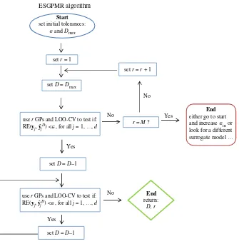
ESGPMR algorithm
Start
set initial tolerances:
Πand Dmax
set r = 1
set r = r + 1
set D = Dmax
set D = D–1 set D = D–1
Yes
No
use r GPs and LOO-CV to test if: RE(yj, yˆjD) <Œ, for all j = 1, …, d
use r GPs and LOO-CV to test if: RE(yj, yˆjD) <Œ, for all j = 1, …, d
End
return:
D, r
r = M ?
No
Yes
Yes
No
End
either go to start and increase Œin or look for a different surrogate model …
Figure 1.ESGPMR algorithm for code implementation.
(i) Set accuracy toleranceεand maximum dimension of the input space to be consideredDmax.
(ii) Setr=1.
(iii) Find a reduced-rank approximationY˜rof the originalYby using the firstrPCs. (iv) SetD=Dmax.
(v) Form the training sets{DiD}ri=1and buildrindependent GPs (as described in §3.2). Follow the leave-one-out cross-validation (LOO-CV) approach and use the previous GPs to predict the fields at the leave-out pointsξˆDj , j=1,. . .,d, and then check if the following expression holds:
RE(yj,yˆDj)< ε, ∀j=1,. . .,d, (3.5)
whereyjare the columns ofY(the true fields) andyˆDj denotes the predicted field at pointξˆDj . If expression (3.5) does not hold, set r=r+1 and go to (iii) (to refine the reduced-rank approximation error). If expression (3.5) holds, setD=Dmax−1 and go to (v) (to reduce the
dimension of the input space) until the expression does not hold, and then returnDandr.
Note that the choices ofεandDmaxare problem-dependent and completely heuristic. In the next
section, we will discuss how to choose values for those tolerances by examining the data, although this ultimately depends on the end-user criteria.
3.4. Leave-one-out cross-validation and hyperparameters estimation
Estimates of the unknown hyperparametersθθθ=(σ2
f,,σn2) in expression (3.1) need to be inferred from
9
rsos
.ro
yalsociet
ypublishing
.or
g
R.
Soc
.open
sc
i.
5
:1
71933
...
cross-validation (LOO-CV) (see [5,21]). LOO-CV consists of using all training set data but one point (the
leave-out) for training, and computing the model prediction error on the leave-out point. This process is repeated until all availabledpoints have been exhausted. We use each of thedleave-out training sets and a conjugate gradient optimizer to obtain estimates of the hyperparameters by maximizing the log marginal likelihood (3.6) with respect to the hyperparameters:
logp(y|X,θθθ)= −1 2y
(Σ+σ2 nI)−1y−
1
2log|Σ+σ
2 nI| −
n
2log 2π. (3.6)
The prediction errors during the LOO-CV scheme are quantified through the mean square error (MSE):
MSE=1
d
d
j=1
(yj−mj)2, (3.7)
wheremjis the predicted expected value given by expression (3.2) andyjis the corresponding observed
value both at the same (leave-out) inputξˆj. Note that the MSE depends only on the mean predictions,
and thus, sometimes, different CV measures which also take into account predictive variances, such as the negative log validation density loss [21] or the Dawid score [52], might be preferred. For the purpose of this study, the MSE gives us the relevant information about the LOO-CV predictions we need for assessment. For an optimal performance of the optimization algorithm and for avoiding failure due to the existence of possible marginal likelihood multiple optima, a continuation routine must be included in all the independent GP emulators described earlier. This is straightforward and can be implemented as follows:
(i) Consider the training sets as in §3.3, i.e. for any D≤M: {DiD=(XD,αi)}ri=1. Without loss of
generality, let us setr=1. The method is exactly the same for the otherr−1 GPs.
(ii) Estimate the hyperparameters by finding the MLE of expression (3.6) for theDone-dimensional problems until a maximum valueDmax(large), i.e. by using theDth KL coefficient of each of the
ddesign points in the training set. We obtainθθθ(ini)=(σf(ini),(ini)1 ,. . .,(ini)D ,σn(ini)). Note that the
importance here lies in the length scales arising from the anisotropic covariance function. Note also that we do not need to compute these valuesa prioriand we can do each calculation just before each iteration as needed (depending onDmax).
(iii) Start the iteration over the number of KL coefficientsD. ForD=1 perform a LOO-CV scheme by using the values obtained in (ii) as initial guess for the estimation of hyperparameters to be used in the GP. Store the hyperparameters asθθθ(1)=(σ(1)
f , (1) 1 ,σ
(1) n ).
(iv) Repeat the iterations untilD=Dmax, and forD>2 take as initial guess the previous estimation
of the hyperparameters in the lower-dimensional space and the first estimation obtained in (ii) for the next component. For example, forθθθ(2)take as initial guess: (σf(1),(1)1 ,(ini)2 ,σn(1)).
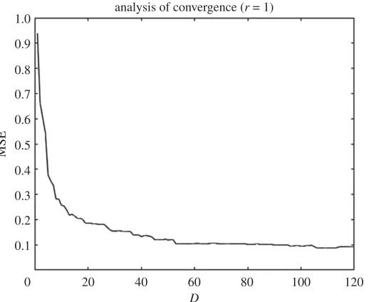
Store the MSE for all theDiterations to examine convergence. By inspectingfigure 2, we can estimate a value forDmaxand refine the model.
4. Numerical results
In this section, we discuss the results obtained by applying the reduction and GP emulation methods to the model problem introduced in §2. Let us consider the numerical simulators fc:ξ→CandfΨ:
ξ→Ψ with ξ∈RM, distributed according toN(0,I).C∈RM andΨ ∈RM are the concentration and streamfunction, respectively. Let us show how we build the GP emulator for the concentration simulator
fc. Exactly the same procedure applies tofΨ. The first step is to build a training set. We generated=256 points as described in §3.1, i.e. we use a Sobol sequence to generatedpoints in [0, 1]M, and, second, push thedpoints component wise through the inverse cumulative distribution function ofMrandom variables distributed according toN(0,σd2), withσd=1.32, to, jointly, form the set of design pointsξˆj, j=1,. . .,d.
For the choice ofσd, we tested the GP simulator for three different values:σd=1.32 was the one providing
more accuracy in the LOO-CV test. To exploit the properties of Sobol sequences and spread the points in the space in an optimal manner, it is recommended [53] that the generated samples are a power of 2. In this study, we used=28=256. A lower number of design points might be used with the same degree of
10
rsos
.ro
yalsociet
ypublishing
.or
g
R.
Soc
.open
sc
i.
5
:1
[image:11.522.136.402.42.254.2] [image:11.522.56.467.348.411.2]71933
...
1.0
0.9
0.8
0.7
0.6
0.5
0.4
0.3
0.2
0.1
0 20 40 60 80 100 120
D
MSE
analysis of convergence (r = 1)
Figure 2.MSE against the number of KL coefficients or input space dimensionD. These data correspond to the emulation of the first PC
component.
Table 1.Relative errors between the true and reduced-rank approximation REtrue-redand between and the true and the predicted
concentration fields REtrue-predfor three different tolerancesε. The numbers of PCs (PC) and KL coefficients (KL) used are also provided.
ε PC KL REtrue-red REtrue-pred
. . . .
0.050 3 5 0.034 0.047
. . . .
0.025 6 14 0.017 0.023
. . . .
0.010 10 82 0.005 0.010
. . . .
The key parameters used to characterize the heterogeneity of the porous medium appeared in expression (2.6). A detailed analysis of the impact of heterogeneity on the concentration profiles and the streamfunction fields has been conducted previously [5,24]; in these earlier works, a measure of the amount of CO2adsorbed through the top boundary in a process of CO2storage is computed from both
the heterogeneous case and the one for an equivalent homogeneous medium characterized by a constant permeability equal to the mean permeability in the domain. For our simulations, the value ofλwill be set toλ=0.5. This value has been taken from the ranges suggested in the literature (see [18]). The existence of bifurcating branches of solutions in the C-ED model (see [32]), i.e. there is not always guarantee of a unique observed value at a single design point, might lead to inaccurate training data if large values ofσ2
are considered and no classification techniques are employed [5]. Thus, for simplicity and without loss of generality, we will setσ2=0.1. Note that the choice ofσ2does not directly affect the applicability of the ESGPMR method proposed in this paper but the uniqueness of the simulator outputs. Consequently, the use of larger values forσ2would probably necessitate using additional pre-processing tools to classify the variety of branches of observed data before forming the training set. This scenario has been treated in detail previously [5]. Note that for models where there is a one-to-one correspondence between inputs and outputs, the ESGPMR can be applied without restriction.
11
rsos
.ro
yalsociet
ypublishing
.or
g
R.
Soc
.open
sc
i.
5
:1
[image:12.522.133.390.42.256.2] [image:12.522.107.419.316.553.2] [image:12.522.52.468.644.709.2]71933
...
1.0
0.9
0.8
0.7
0.6
0.5
0.4
0.3
0.2
0.1
0 2 4 6 8 10 12
MSE
r
analysis of convergence (D = 120)
Figure 3.MSE against the number of PCs or output space dimensionr. These data correspond to a GP emulation withD=120.
1.0
0.8
0.6
0.4
–0.4 0.2
–0.2 0
–0.6
–0.8
–1.0
0 0.5 1.5 0.4113
0.6218 0.8323 1.0429 1.2534 1.4639 1.6744 1.8849 2.0954
1.0
z
x
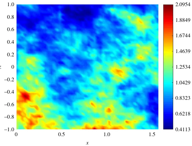
Figure 4.Permeability field used for the prediction of the concentration and streamfunction fields shown in figures5and6.
Table 2.Relative errors between the true and reduced-rank approximation REtrue-redand between and the true and the predicted
streamfunction fields REtrue-predfor three different tolerancesε. The numbers of PCs (PC) and KL coefficients (KL) used are also provided.
ε PC KL REtrue-red REtrue-pred
. . . .
0.100 5 6 0.069 0.095
. . . .
0.075 10 18 0.036 0.072
. . . .
0.050 14 55 0.017 0.048
12
rsos
.ro
yalsociet
ypublishing
.or
g
R.
Soc
.open
sc
i.
5
:1
[image:13.522.141.381.40.603.2]71933
...
true concentration field
reduced-rank field (r = 10, D = 82, RE = 0.005)
emulated field (r = 10, D = 82, RE = 0.01) 1.0
0.9
0.8
0.7
0.6
0 0.2 0.4 0.6 0.8 1.0
0.2 0.4 0.6 0.8 1.0
0.2 0.4 0.6 0.8 1.0
0.1 0.2 0.3 0.4 0.5
1.0
0.9
0.8
0.7
0.6
0.1 0.2 0.3 0.4 0.5 1.0
0.9
0.8
0.7
0.6
0.1 0.2 0.3 0.4 0.5 1.0
0.9
0.8
0.7
0.6
0.1 0.2 0.3 0.4 0.5
z
1.0
0.9
0.8
0.7
0.6
0 0.1 0.2 0.3 0.4 0.5
z
1.0
0.9
0.8
0.7
0.6
0 0.1 0.2 0.3 0.4 0.5
z
x x x
(b) (a)
(c)
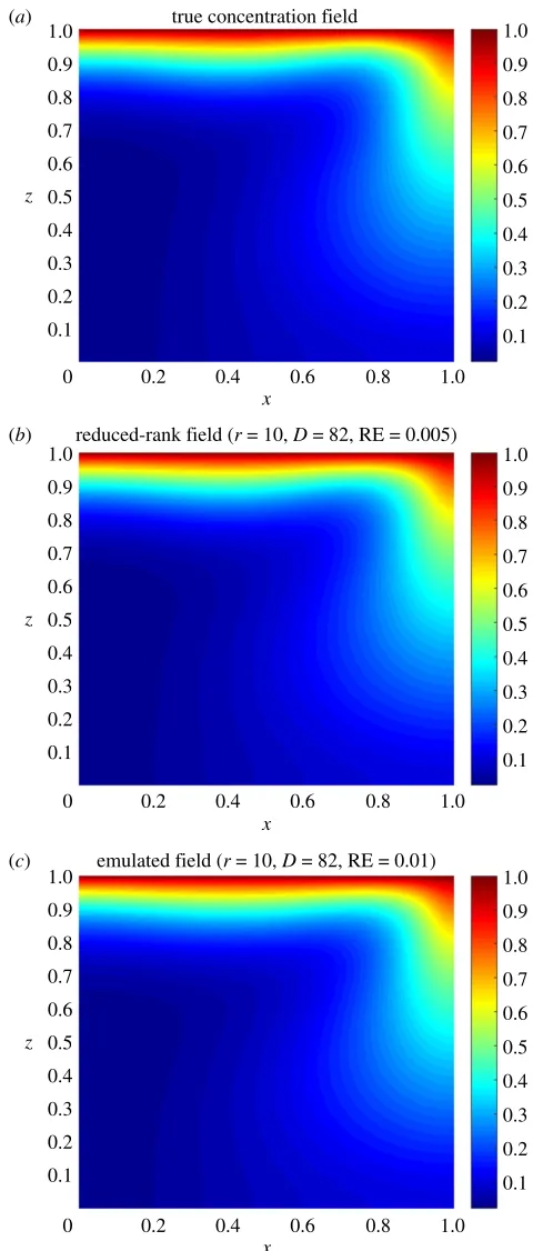
Figure 5.True (a), reduced rank (b) and predicted (c) concentration fields for the permeability shown infigure 4. The dimension of the
input (D) and output (r) spaces and the relative error (RE) achieved are also reported.
designed. To set an optimal value forDmax, we need to conduct a first experiment allowing Dmax to
be large enough to allow us to investigate, for instance by visual inspection, some signs or numerical evidence of convergence. Figure2provides us with a valuable information about the latter. For this model, a sensible value forDmaxmight be 100 (higher or lower values are at user discretion). Note that
13
rsos
.ro
yalsociet
ypublishing
.or
g
R.
Soc
.open
sc
i.
5
:1
71933
...
1.0
0.9
0.8
0.7
0.6
0 0.2 0.4 0.6 0.8 1.0
0.2 0.4 0.6 0.8 1.0
0.2 0.4 0.6 0.8 1.0
0.1 0.2 0.3 0.4 0.5
z
1.0
0.9
0.8
0.7
0.6
0 0.1 0.2 0.3 0.4 0.5
z
x x x
(b)
(c)
true streamfunction field
reduced-rank field (r = 14, D = 55, RE = 0.017)
emulated field (r = 14, D = 55, RE = 0.048) 1.0
0.9
0.8
0.7
0.6
0 0.1 0.2 0.3 0.4 0.5
z
(a)
–0.06 –0.05 –0.04 –0.03 –0.02 –0.01 0
–0.06 –0.05 –0.04 –0.03 –0.02 –0.01 0
–0.06 –0.05 –0.04 –0.03 –0.02 –0.01 0
Figure 6.True (a), reduced rank (b) and predicted (c) streamfunction fields for the permeability shown infigure 4. The dimension of the
input (D) and output (r) spaces and the relative error (RE) achieved are also reported.
the value ofDmaxis just a reference, using more DoF does not seem to be sensible as it could lead to
additional numerical errors as well as an exponential increase of the computational cost. It is important to note thatDmaxis just a user’s auto-imposed limit depending on the user’s own computational resources,
14
rsos
.ro
yalsociet
ypublishing
.or
g
R.
Soc
.open
sc
i.
5
:1
[image:15.522.134.398.38.255.2]71933
...
scatterplot of 256 points based on D = 82 and r = 10 0.75
0.70
0.65
0.60
0.55
0.50
0.45
0.45 0.50 0.55 0.60 0.65 0.70 0.75 predicted
observ
ed
Figure 7.Scatterplot of the massMcomputed from the 256 observed concentration fields in the training set and the predicted mass
obtained from the emulated concentration fields at the same design points. The liney=xis used as the reference for the best possible performance.
desired accuracy in the GP predictions for either a toleranceεor a relatively large value ofDmax, it can
be concluded that GP emulation is nota priori(one can always try with different prior mean, covariance or likelihood functions) a recommendable surrogate model for the numerical simulator. Figure3shows numerical evidence of how the reduction of the MSE depends on the number of PCs considered.Figure 4 shows the permeability field used to compute the concentration and the streamfunction outputs shown in figures5and6. Figure5shows the results obtained by using the GP emulator withD=82 andr=10 to predict the concentration output field at one untested pointξ∗∈RM. The RE between the true and the reduced rank approximation was 0.005. The RE between the true and the predicted was 0.01. Figure6 shows the results for the same input considered infigure 5, where in this case the best resolution achieved was usingD=55 andr=14. We highlight here that different values ofDandrare needed for each GP emulator to achieve the desired tolerance, i.e. while for the concentration we neededD=5 and r=3 to achieve a tolerance of 0.05, for the streamfunction we neededD=55 andr=14. Furthermore, both algorithms were unable to refine further, and thus the lowest tolerances we could achieve in this study wereε=0.01 for the concentration andε=0.05 for the streamfunction.
Before finishing this section, let us see another application. We can use the GP emulator to approximate scalar-valued quantities of interest from any of the output fields, for instance we can compute the total mass of dissolved solute in the domainRgiven by BarbaRossaet al. [34]:M=RC. In this case, we only need to emulate the concentration fieldCfor the new input and then compute the integral overR. An intuitive and qualitative way of measuring how close our GP predictions are to the observed values is through scatterplots. This consists of plotting the pairs (predicted outputs, observed outputs) along with the liney=xand checking that the scattered points are not ‘far away’ from the straight line. For this application, we used the data stored during the LOO-CV scheme for the GP above and computed the setM∗1,. . .,M∗dfrom the emulated concentration fields. Then we computed
M1,. . .,Mddirectly from the simulator concentration outputsC1,. . .,Cd. Figure7shows the scatterplot
for the observed values (Y-axis) against the predicted values (X-axis).
In this study, the GP emulation was implemented using the GPML MATLAB TOOLBOXv.3.4 [21].
5. Conclusion
15
rsos
.ro
yalsociet
ypublishing
.or
g
R.
Soc
.open
sc
i.
5
:1
71933
...for the emulation of concentration fields, one of the GP emulators was able to reduce the dimensionality of the input and output spaces fromM=2601 toD=112 and fromM=2601 tor=20, respectively, for an overall tolerance ofε=0.01.
The ESGPMR algorithm provides the end-user with a tool for assessing if GP emulation is an efficient surrogate model for a given computationally expensive numerical simulator. This applies to either numerical models where it is not feasible to meet the desired resolution in the GP predictions or when the original problem cannot be adequately reduced to a more tractable model (i.e.Dmaxandrare found
to be extremely large for the tolerances given).
Data accessibility. Our data are available in Dryad athttps://doi.org/10.5061/dryad.3g280[54].
Competing interests. The author declares that there are no competing interests.
Funding. This research was funded by the EU Panacea project, FP7, grant agreement 282900.
References
1. Byers E, Stephens DB. 1983 Statistical and stochastic analyses of hydraulic conductivity and particle-size in a fluvial sand.Soil Sci. Soc. Am. J.47, 1072– 1081. (doi:10.2136/sssaj1983.036159950047000 60003x)
2. Hoeksema RJ, Kitanidis PK. 1985 Analysis of the spatial structure of properties of selected aquifers. Water Resour. Res.21, 536–572. (doi:10.1029/ WR021i004p00563)
3. Russo D, Bouton M. 1992 Statistical analysis of spatial variability in unsaturated flow parameters. Water Resour. Res.28, 1911–1925. (doi:10.1029/ 92WR00669)
4. Mondal A, Efendiev Y, Mallick B, Datta-Gupta A. 2010 Bayesian uncertainty quantifcation for flows in heterogeneous porous media using reversible jump Markov chain monte carlo methods.Adv. Water Resour.33, 211–256. (doi:10.1016/j.advwatres. 2009.10.010)
5. Crevillen-Garcia D, Wilkinson RD, Shah AA, Power H. 2017 Gaussian process modelling for uncertainty quantification in convectively-enhanced dissolution processes in porous media.Adv. Water Resour.99, 1–14. (doi:10.1016/j.advwatres.2016.11.006) 6. Mara TA, Fajraoui N, Guadagnini A, Younes A. 2017
Dimensionality reduction for efficient Bayesian estimation of groundwater flow in strongly heterogeneous aquifers.Stoch Environ. Res. Risk Assess.31, 2313–2326. doi:10.1007/s00477-016-1344-1)
7. Crevillen-Garcia D, Power H. 2017 Multilevel and quasi-Monte Carlo methods for uncertainty quantification in particle travel times through random heterogeneous porous media.R. Soc. open sci.4, 170203. (doi:10.1098/rsos.170203) 8. Rabitz H, Aliş OF, Shorter J, Shim K. 1999 Efficient
input-output model representations.Comput. Phys. Commun.117, 11–20. (doi:10.1016/
S0010-4655(98)00152-0)
9. Rabitz H, Aliş OF. 1999 General foundations of high-dimensional model representations.J. Math. Chem.25, 197–233. (doi:10.1023/A:
1019188517934)
10. Aliş OF, Rabitz H. 2001 Efficient implementation of high dimensional model representations.J. Math. Chem.29, 127–142. (doi:10.1023/A:1010979129659) 11. Ma X, Zabaras N. 2010 An adaptive
high-dimensional stochastic model representation technique for the solution of stochastic partial differential equations.J. Comput. Phys.229, 3884–3915. (doi:10.1016/j.jcp.2010.01.033)
12. He X, Jiang L, Moulton JD. 2013 A stochastic dimension reduction multiscale finite element method for groundwater flow problems in heterogeneous random porous media.J. Hydrol. 478, 77–88. (doi:10.1016/j.jhydrol.2012.11.052) 13. Xiu D, Hesthaven JS. 2005 High-order collocation
methods for differential equations with random inputs.SIAM J. Sci. Comput.27, 1118–1139. (doi:10.1137/040615201)
14. Babuška I, Nobile F, Tempone R. 2007 A stochastic collocation method for elliptic partial differential equations with random input data.SIAM. J. Numer. Anal.45, 1005–1034. (doi:10.1137/050645142) 15. Ganapathysubramanian B, Zabaras N. 2007 Sparse
grid collocation schemes for stochastic natural convection problems.J. Comput. Phys.225, 652–685. (doi:10.1016/j.jcp.2006.12.014) 16. Nobile F, Tempone R, Webster CG. 2008 A sparse
grid stochastic collocation method for partial differential equations with random input data. SIAM. J. Numer. Anal.46, 2309–2345. (doi:10. 1137/060663660)
17. Ganapathysubramanian B, Zabaras N. 2007 Modeling diffusion in random heterogeneous media: data-driven models, stochastic collocation and the variational multiscale method.J. Comput. Phys.226, 326–353. (doi:10.1016/j.jcp.2007.04.009) 18. Cliffe KA, Giles MB, Scheichl R, Teckentrup AL. 2011 Multilevel Monte Carlo methods and applications to elliptic PDEs with random coefficients.Comput. Visual Sci.14, 3–15. (doi:10.1007/s00791-011-0160-x) 19. Sacks J, Welch WJ, Mitchell TJ, Wynn HP. 1989
Design and analysis of computer experiments.Stat. Sci.4, 409–423.
20. O’Hagan A. 1992 Some Bayesian numerical analysis. Bayesian Stat.4, 345–363.
21. Rasmussen CE, Williams CKI. 2006Gaussian processes for machine learning. Cambridge, MA: MIT Press.
22. Bowman VE, Woods DC. 2016 Emulation of multivariate simulators using thin-plate splines with application to atmospheric dispersion. SIAM/ASA J. Uncertain. Quantification4, 1323–1344. (doi:10.1137/140970148)
23. Jalobeanu A, Blanc-Féraud L, Zerubia J. 2002 Hyperparameter estimation for satellite image restoration using a MCMC maximum-likelihood method.Pattern Recognit.35, 341–352. 24. Crevillen-Garcia D. 2016 Uncertainty quantification
for flow and transport in porous media. PhD Thesis, University of Nottingham, UK.
25. Neal RM. 1996Bayesian learning for neural networks. Lecture Notes in Statistics, vol. 118. New York, NY: Springer.
26. Higdon D, Gattike J, Williams B, Rightley M. 2008 Computer model calibration using high-dimensional output.J. Am. Stat. Assoc.103, 570–583. (doi:10.1198/016214507000000888) 27. Holden PB, Edwards NR, Garthwaite PH, Wilkinson
RD. 2015 Emulation and interpretation of high-dimensional climate model outputs.J. Appl. Stat.42, 2038–2055. (doi:10.1080/02664763. 2015.1016412)
28. IPCC. Fifth Assessment Report (AR5). Intergovernmental Panel on Climate Change. Seehttps://www.ipcc-wg2.gov/AR5-tools/. 29. Cliffe KA, Spence A, Tavener SJ. 2000 The numerical
analysis of bifurcation problems with application to fluid mechanics.Acta Numer.9, 39–131. 30. Ghesmat K, Hassanzadeh H, Abedi J. 2011 The
impact of geochemistry on convective mixing in a gravitationally unstable diffusive boundary layer in porous media: CO2storage in saline aquifers.J. Fluid Mech.673, 480–512. (doi:10.1017/
S0022112010006282)
31. Neufeld JA, Hesse MA, Riaz A, Hallworth MA, Tchelepi HA, Huppert HE. 2010 Convective dissolution of carbon dioxide in saline aquifers. Geophys. Res. Lett.37, L22404. (doi:10.1029/ 2010GL044728)
32. Ward TJ, Cliffe KA, Jensen OE, Power H. 2014 Dissolution-driven porous-medium convection in the presence of chemical reaction.J. Fluid Mech. 747, 316–349. (doi:10.1017/jfm.2014.149) 33. Ranganathan P, Farajzadeh R, Bruining H, Zitha PLJ.
2012 Numerical simulation of natural convection in heterogeneous porous media for CO2geological storage.Transp. Porous Med.95, 25–54. (doi:10.1007/s11242-012-0031-z)
34. BarbaRossa G, Cliffe KA, Power H. 2017 Effects of hydrodynamic dispersion on the stability of buoyancy driven porous-media convection in the presence of first order chemical reaction.J. Eng. Math.103, 55–76. ( doi:10.1007/s10665-016-9860-z)
35. Saffman PG. 1959 A theory of dispersion in a porous medium.J. Fluid Mech.6, 321–349. (doi:10.1017/ S0022112059000672)
16
rsos
.ro
yalsociet
ypublishing
.or
g
R.
Soc
.open
sc
i.
5
:1
71933
...
37. Hidalgo J, Carrera J. 2009 Effect of dispersion on the onset of convection during CO2sequestration.J. Fluid Mech.640, 441–452. (doi:10.1017/ S0022112009991480)
38. Xie Y, Simmons CT, Werner AD, Diersch H-JG. 2012 Prediction and uncertainty of free convection phenomena in porous media.Water Resour. Res.48, W02535. (doi:10.1029/2011WR011346) 39. Brenner SC, Scott LR. 2008The mathematical theory
of finite element methods. New York, NY: Springer-Verlag.
40. Antonietti P, Giani S, Hall E, Houston P, Krahl R. 2013 Aptofem. Finite element software toolkit. University of Nottingham, School of Mathematics. See
https://www.maths.nottingham.ac.uk/personal/ph/ Site/Software.html
41. Amestoy PR, Duff IS, L’Excellent J-Y, Koster J. 2001 A fully asynchronous multifrontal solver using distributed dynamic scheduling.SIAM J. Matrix Anal. Appl.23, 15–41. (doi:10.1137/S089547989935 8194)
42. Amestoy PR, Guermouche A, L’Excellent J-Y, Pralet S. 2006 Hybrid scheduling for the parallel solution of linear systems.Parallel Comput.32,
136–156. (doi:10.1016/j.parco.2005. 07.004)
43. Dentz M, LeBorgne T, Englert A, Bijeljic B. 2011 Reactive transport and mixing in heterogeneous media: a brief review.J. Contam. Hydrol120-121, 1–17. (doi:10.1016/j.jconhyd.2010.05.002) 44. Collier N, Haji-Ali A-L, Nobile F, von Schwerin E,
Tempone R. 2014 A continuation multilevel Monte Carlo algorithm.BIT Numer. Math.55, 399–432. (doi:10.1007/s10543-014-0511-3)
45. Stone N. 2011 Gaussian process emulators for uncertainty analysis in groundwater flow. PhD Thesis, University of Nottingham, UK. 46. Lord GJ, Powell CE, Shardlow T. 2014An introduction
to computational stochastic PDEs. Cambridge texts in Applied Mathematics. Cambridge, UK: Cambridge University Press.
47. Ghanem R, Spanos D. 1991Stochastic finite element: a spectral approach. New York, NY: Springer. 48. Strang G. 2003Introduction to linear algebra. Cambridge, MA: Wellesley-Cambridge Press. 49. McKay MD, Beckman RJ, Conover WJ. 1979 A
comparison of three methods for selecting values of input variables in the analysis of output from a
computer code.Technometrics21, 239–245. (doi:10.2307/1268522)
50. Pebesma EJ, Heuvelink GBM. 1999 Latin hypercube sampling of Gaussian random fields.Technometrics 41, 303–312. (doi:10.1080/00401706.1999.1048 5930)
51. Sobol IM. 1967 On the distribution of points in a cube and approximate evaluation of integrals. Comput. Maths. Math. Phys.7, 86–112. (doi:10. 1016/0041-5553(67)90144-9)
52. Dawid AP, Sebastiani P. 1999 Coherent dispersion criteria for optimal experimental design.Ann. Stat. 27, 65–81.
53. Burhenne S, Jacob D, Henze GP. 2011 Sampling based on sobol sequences for Monte Carlo techniques applied to building simulations. InProc. Building Simulation 2011: 12th Conf. of Int. Building Performance Simulation Association, Sydney, 14–16 November, pp. 1816–1823.