arXiv:1802.06580v3 [cond-mat.dis-nn] 13 Apr 2018
Desynchronization induced by time-varying network
Maxime Lucas,1, 2,∗ Duccio Fanelli,2,† Timoteo Carletti,3,‡ and Julien Petit3, 4,§ 1
Department of Physics, Lancaster University, Lancaster LA1 4YB, United Kingdom 2
Dipartimento di Fisica e Astronomia, Universit`a di Firenze, INFN and CSDC, Via Sansone 1, 50019 Sesto Fiorentino, Firenze, Italy 3
naXys, Namur Institute for Complex Systems, University of Namur, B5000 Namur, Belgium 4
Department of Mathematics, Royal Military Academy, B1000 Brussels, Belgium
(Dated: April 16, 2018)
The synchronous dynamics of an array of excitable oscillators, coupled via a generic graph, is studied. Non homogeneous perturbations can grow and destroy synchrony, via a self-consistent instability which is solely instigated by the intrinsic network dynamics. By acting on the char-acteristic time-scale of the network modulation, one can make the examined system to behave as its (partially) averaged analog. This result if formally obtained by proving an extended version of the averaging theorem, which allows for partial averages to be carried out. As a byproduct of the analysis, oscillation death are reported to follow the onset of the network driven instability.
Natural and artificial systems are often composed of individual oscillatory units, coupled together so as to yield complex collective dynamics [1–5]. Weak coupling of non-linear oscillators leads to synchronization [4], a condition of utmost coordination which is eventually met when the parts of a system operate in unison. Syn-chronization has been addressed theoretically in a wide range of settings, climbing the hierarchy of complexity from simple unidirectionally phase forced oscillator, with a fixed frequency [4] and more recently a time-varying frequency [6, 7], to large populations of mutually inter-acting, individually oscillating, entities [2]. The simulta-neous flashing of fireflies and the rhythmic applause in a large audience are representative examples both ascrib-able to the vast and multifaceted realm of synchroniza-tion phenomena [5]. Synchronisation of self-sustained os-cillators on complex networks has attracted considerable interest in the last decade, the emphasis being primar-ily placed on the pivotal role exerted by the topology of the graph that shapes the underlying couplings [8,9]. Other studies elaborated on the effect produced by im-posing an external perturbation, such as noise [10], a (fixed-frequency) pacemaker forcing [11,12], or more re-cently an external modulation of frequencies [13–15]. De-lays in the network of couplings have been also enforced and their impact on the synchronizability property thor-oughly assessed [16].
At the other extreme entirely, when the coupling strength is made to increase, oscillations may go ex-tinct. Oscillation death is observed in particular when an initially synchronized state evolves torwards an asymp-totic inhomogeneous steady configuration [17–20], in re-sponse to an externally injected perturbation [21]. Un-derstanding the mechanisms that drive the suppression of the oscillations in spatially extended systems,
assim-∗[email protected] †[email protected] ‡[email protected] §[email protected]
ilated to disordered networks, may prove to be relevant for e.g. neuroscience applications. The ability of disrupt-ing synchronous oscillations could be in fact exploited as a dynamical regulator [22–24], to oppose pathologi-cal neuronal states that are found to consistently emerge in Alzheimer and Parkinson diseases. Landscape frag-mentation and then dispersal among connected patches sits at the origin of oscillation death in ecology, with its noteworthy fallout in terms of diversity and stability [25]. To date, oscillation death has been mostly analyzed on static networks. In many cases of interests [26–28], how-ever, links are intermittently active and signals can crawl only when connections are functioning: diseases spread through physical proximity, pathogens flowing therefore on dynamic contact graphs; neural and brain networks can be also represented as time-varying graphs, resources driven activation playing a role of paramount impor-tance.
The inherent ability of a network to adjust in time acts as a veritable non-autonomous drive. In a recent Letter [29], the process of pattern formation for a mul-tispecies model anchored on a time-varying network was analyzed. It was in particular shown that a homogeneous stable fixed point can turn unstable, upon injection of a non-homogeneous perturbation, via a symmetry break-ing instability which is reminiscent of the Turbreak-ing mech-anism [30], but solely instigated by the intrinsic network dynamics. Starting from these premises, the aim of this work is to extend the theory presented in [29] to the rel-evant setting where the unperturbed homogeneous solu-tion typifies as collecsolu-tion of synchronized limit-cycles. In other words, we will set to analyze how the synchrony of a large population of non-linear, diffusively coupled oscilla-tors may be disrupted by network plasticity. Surprisingly, oscillation death can be induced by a piecewise constant time-varying network, also when synchrony is guaranteed on each isolated network snapshot. Our analysis provides a solid theoretical backup to the work of [31], where the oscillation death phenomenon is numerically observed on fast time-varying networks.
evolves over time and denote byxiandyitheir respective
concentrations, as seen on nodei. The structural prop-erties of the (symmetric) network are stored in a time-varying N×N weighted adjacency matrix Aij(t). For
the ease of calculation, we will hereafter assumeN con-stant. Introduce the Laplacian matrixLwhose elements readLij(t) =Aij(t)−Ki(t)δij, whereKi(t) =PjAij(t)
stands for the connectivity of nodei, at timet. The cou-pled dynamics of xi and yi, for i= 1, ..., N, is assumed
to be ruled by the following, rather general equations:
˙
xi=f(xi, yi) +Dx N
X
j=1
Lij(t/ǫ)xj,
˙
yi=g(xi, yi) +Dy N
X
j=1
Lij(t/ǫ)yj,
(1)
where Dx and Dy are appropriate coupling parameters.
Here, f and g are non-linear reaction terms, chosen in such a way that system (1) exhibits a homogeneous sta-ble solution (xi, yi)≡(¯x(t),y¯(t))∀iwhich is periodic of
periodT. To state it differently, whenDx=Dy= 0, the
above system is equivalent toN identical replica of a two dimensional deterministic model, which displays a stable limit-cycle. The homogeneous time-dependent solution obtained for Dx 6= 0 6= Dy, when setting in phase the
self-sustained oscillations on each node of the collection, corresponds to the synchronized regime that we shall be probing in the forthcoming investigation. The parame-ter ǫ controls the time-scale of the Laplacian dynamics. We will specifically inspect the case of a network that is periodically rearranged in time and denote with Ts the
period of the network modulation, as obtained forǫ= 1. By operating in this context, we will show that synchro-nization can be eventually lost when forcing ǫ below a critical threshold. When successive swaps between two static network configurations are considered over one pe-riod Ts (as it is the case, in the example addressed in
the second part of the paper), ǫ sets the frequency of the blinking. The extension to non-periodic settings is straightforward, as discussed in details in [29].
To proceed with the analysis we compactify the notation by introducing the 2N-element vector x = (x1, . . . , xN, y1, . . . , yN)T. The dynamics of the system
can be hence cast in the form:
˙
x=F(x) +L(t/ǫ)x, (2)
where F(x) = (f(x1, y1), . . . , f(xN, yN), g(x1, y1), . . . ,
g(xN, yN))T; the 2N×2Nblock diagonal matrixLreads:
L(t) =
DxL(t) 0
0 DyL(t)
. (3)
As mentioned above, the non-linear reaction terms, now stored in matrixF, are chosen so as to have a stable limit-cycle in the uncoupled setting Dx =Dy = 0. The
stability of the limit-cycle (¯x(t),y¯(t)) can be assessed by
means of a straightforward application of the Floquet theory. To this end, we focus on the two dimensional system obtained in the uncoupled limit and introduce a perturbation of the time-dependent equilibrium, namely δx= (x−x, y¯ −y¯)T. Linearizing the governing equation
yieldsδx˙ =J(t)δx, whereJ(t) =∂xF(x) is periodic of
periodT. Let us label with Φ(t) a fundamental matrix of the system. Then, for allt, there exists a non-singular, constant matrixB such that:
Φ(t+T) = Φ(t)B. (4)
Moreover, detB = exphR0TtrJ(t) dti. The matrix B depends in general on the choice of the fundamental ma-trix Φ(t). Its eigenvalues, ρi with i = 1,2, however, do
not. These are called the Floquet multipliers and yield the Floquet exponents, defined asµi =T−1lnρi.
Solu-tions of the examined linear system can then be written:
x(t) =a1p1(t)eµ1t+a2p
2(t)eµ2t, (5)
where thepi(t) functions areT-periodic, andaiare
con-stant coefficients set by the initial conditions. When the system is linearized about limit-cycles arising from first-order equations, one of the Floquet exponents is iden-tically equal to zero, µ1 = 0. The latter is associated with perturbations along the longitudinal direction of the limit-cycle: these perturbations are neither amplified nor damped as the motion progresses. The other exponent, µ2 takes instead negative real values, if the limit-cycle is stable, meaning that perturbations in the transverse direction are bound to decay in time.
We now turn to discussing the original system (2). The reaction parameters are set so to yield a stable limit-cycle for Dx = Dy = 0. Furthermore, we assume the
oscil-lators to be initially synchronized, with no relative de-phasing. We then apply a small, nonhomogeneous, hence node-dependent perturbation and set to explore the con-ditions which can yield a symmetry breaking instability of the synchronized regime, from which the oscillation death phenomenon might eventually emerge. We are in particular interested in elaborating on the role played by the non-autonomous network dynamics in seeding the aforementioned instability. Introduce a small inhomo-geneous perturbation around the synchronous solution δx= (x1−x, . . . , x¯ N −x, y1¯ −y, . . . , y¯ N−y¯)T, and
lin-earize the governing equation (2) so as to yield:
δx˙ = [J(t) +L(t/ǫ)]δx. (6)
This is a non-autonomous equation, and it is difficult to treat it analytically [32], owing in particular to the simultaneous presence of different periods. To overcome this limitation, and gain analytical insight into the prob-lem under scrutiny, we introduce the averaged Laplacian hLi= 1/Ts
RTs
0 Ldt and define the following system:
˙
As we will rigorously show in the following, the stabil-ity of the synchronous solution of system (2) is eventu-ally amenable to that of system (7). Stated differently, assume that an external non-homogeneous perturbation can trigger an instability in system (7). Then, ǫ∗ ex-ists such that the original system (2) is also unstable for 0 < ǫ < ǫ∗. In other words, by tuning sufficiently small the parameterǫ, and thus forcing a high frequency modulation of the network Laplacian, one can yield a loss of stability of the synchronous solution. Oscillation death can eventually emerge as a possible stationary sta-ble attractor of the ensuing dynamics, promoted by the inherent ability of the network to adjust in time.
As a first step towards proving the results, we shall rescale time asτ=t/ǫ. Eq. (6) can be hence cast in the equivalent form:
δx′=ǫ[(J(ǫτ) +L(τ)]δx, (8)
where the prime denotes the derivative with respect to the new time variableτ. The partially averaged version of (8) [or alternatively the linear version of system (7), after time rescaling], reads δy′ = ǫ[J(ǫτ) +hLi]δy. In the following, we will show thatδy(t)−δx(t)∈ O(ǫ) for up to a time τ ∈ O(1/ǫ), provided that δy(0) = δx(0) and forǫ < ǫ∗. This conclusion builds on a theorem that we shall prove hereafter in its full generality, and which extends the realm of applicability of the usual averaging theorem. Denote x ∈ RΩ, and consider the following equation
˙
x=ǫf1(x, ǫt) +ǫf2(x, t), (9)
where f1(x, t) is T-periodic in t, and f2(x, t) is Ts
-periodic in t. Notice that f1(x, ǫt) is T /ǫ-periodic. It is assumed that f1 and f2 and their derivative are well behaved Lipschitz-continuous functions. Observe inci-dentally that Eq. (8) is recovered by replacing t 7→ τ, x 7→ δx, f1(x, ǫt) 7→ J(ǫτ)δx, f2(x, t) 7→ L(τ)δx and Ω = 2N.
The standard version of the averaging theorem [33] requires dealing with periodic functions, whose periods are independent ofǫ. This is obviously not the case for f1(·, ǫt). To bypass this technical obstacle, we will adapt the proof in [33] to yield an alternative formulation of the theorem which allows for partial averaging to be per-formed. Define:
u(x, t) = Z t
0
ds[f2(x, s)− hf2i], (10)
wherehf2i= 1/Ts
RTs
0 f2(x, t) dtis the average off2over its period. Introduce then thenear-identity transforma-tion
x(t) =z(t) +ǫu(z(t), t), (11)
which yields
˙
x= ˙z+ǫ∂u ∂zz˙+ǫ
∂u
∂t. (12)
Moreover,∂u/∂t(z, t) =f2(z, t)− hf2iby definition ofu, see Eq. (10). Then making use of Eq. (9), it is straight-forward to get:
≡Γ
z }| {
1+ǫ∂u ∂z
˙
z=ǫ[f1(z+ǫu, ǫt) +f2(z+ǫu, t)−f2(z, t) +hf2i],
(13)
Invoking the Lipschitz-continuity off2and the bounded-ness ofuyields :
||f2(z+ǫu, ǫt)−f2(z, ǫt)|| ≤Lǫ||u(z, ǫt)||,
≤LǫM, (14)
whereLandM are positive constants. Hence:
Γ ˙z=ǫf1(z+ǫu, ǫt) +ǫhf2i+O(ǫ2),
≃ǫf1(z, ǫt) +ǫhf2i. (15)
We do not know in general if Γ is invertible, but the identity is and, by continuity, any matrix sufficiently close to it. Hence, there exists a critical valueǫ∗≪1 such that Γ is invertible, if 0< ǫ < ǫ∗. We will return later on pro-viding a self-consistent estimate for the critical threshold ǫ∗. Up to orderO(ǫ), we have:
Γ−1≃
1−ǫ∂u ∂z
. (16)
Hence finally,
˙
z≃ǫ[f1(z, ǫt) +hf2i]. (17)
In conclusion, system (9) behaves like itspartially aver-aged version (17), for times which grow like 1/ǫ, when ǫ is made progressively smaller. Back to the examined model, system (8) stays thus close to its partially aver-aged homologue:
δy′=ǫ[J(ǫτ) +hLi]δy, (18)
which, in terms of the original time scalet amounts to:
δy˙ =M(t)δy, (19)
System (19) can be conveniently studied by expand-ing the perturbation on the basis of the average Lapla-cian operator,hLi= 1/Ts
RTs
0 Ldt [34]. Introduce φ (α),
such that PNj=1hLiijφj(α) = Λαφ(iα), where Λα stands
for the eigenvalues of hLi and α = 1, . . . , N. Note that the eigenvectors are time-independent, as the av-eraged network (hence, the Laplacian) is. Write then δxi(t) = P
N α=1c
x α(t)φ
(α)
i and δyi(t) = P N α=1c
y α(t)φ
(α)
i ,
where cx
α and cyα encode the time-evolution of the
lin-ear system [19, 35, 36]. Plugging the above ansatz into equation (19) yields the following consistency condition:
˙
cα=Mα(t)cα, (20)
where cα = (cxα, cyα)T, and Mα(t) = J(t) +
Λα
Dx 0
0 Dy
. The fate of the perturbation is
deter-mined upon solving the above 2×2 linear system, for each Λα. To this end, remark that Mα is periodic,
with period T,∀α. Solving system (20) amounts there-fore to computing the Floquet exponentsµ(1α) and µ(2α), for α = 1, . . . , N. The dispersion relation is obtained by selecting the largest real part of µ(iα), i = 1,2, at
fixed α [20]. For undirected networks (Aij = Aji), the
Laplacian is symmetric and the Λα are real and
non-positive [37]. For α = 1 the largest Floquet multiplier is zero, since the model displays in its a-spatial version (Λ1 = 0) a stable limit-cycle. We then sort the indices (α) in decreasing order of the eigenvalues, so that the condition 0 = Λ1 ≥Λ2≥... ≥ΛN holds. If the
disper-sion relation is negative ∀ Λα with α > 1, the imposed
perturbation fades away exponentially: the synchronous solution is therefore recovered, for both the average sys-tem (19), and its original analogue, in light of the above analysis, and for allǫ. Conversely, if the dispersion rela-tion takes positive values, even punctually, in correspon-dence of specific Λα, belonging to its domain of definition,
then the perturbation grows exponentially in time, for ǫ smaller than a critical threshold. The initial synchrony for the original system (2) is hence lost and patterns may emerge.
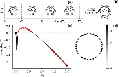
To clarify the conclusion reached above, we shall here-after consider a pedagogical example, borrowed from [29]. Introduce the Brusselator model, a universally accepted theoretical playground for exploring the dynamics of au-tocatalytic reactions. This implies selecting f(x, y) = 1−(b+ 1)x+cx2y andg(x, y) =bx−cx2y, whereb and cstand for free parameters. Forb > c+ 1, the Brussella-tor model displays a limit-cycle. Following, [29] we then consider two networks, made of an even number, N, of nodes arranged on a periodic ring, and label their associ-ated adjacency matricesA1andA2, respectively. Nodes are connected in pairs, via symmetric edges. When it comes to the network encoded in A1, the couples are formed by the nodes labelled with the indexes 2k−1 and 2kfork= 1,2, ..., N/2 [see panel (a) in Fig.1]. The net-work specified via the adjacency matrixA2 links nodes 2k and 2k+ 1, with the addition of nodes 1 and N [as
depicted in panel (a) in Fig. 1]. Both networks return an identical Laplacian spectrum, namely two degenerate eigenvalues Λ1= 0 and ΛN =−2, with multiplicityN/2.
The parameters of the Brussellator are set so that the synchronized solution is stable on each network, taken independently. This is illustrated in panel (c) of Fig. 1, where the corresponding dispersion relation (largest real part of the Floquet multipliers vs. −Λα) is plotted with
black star symbols. Introduce now the time-varying net-work, specified by the adjacency matrixA(t), defined as:
A(t) =
A1 if mod (t, Ts)∈[0, γ[,
A2 if mod (t, Ts)∈[γ,1[, (21)
whereγ (resp. 1−γ) is the fraction of Ts that the
net-work spends in the configuration specified by the ad-jacency matrix A1 (resp. A2). The average network is hence characterized by the adjacency matrix hAi = γA1+ (1−γ)A2, see panel (b) in Fig.1. We then set to consider the stability of the synchronized state in pres-ence of a time-varying network, and resort to its static, averaged counterpart. The average network Laplacian has many more distinct eigenvalues, and these latter fall in a region where the largest real part of the Floquet ex-ponents is positive, as can be appreciated in Fig.1, panel (c), thus signaling the instability. The solid line stands for the dispersion relation that is eventually recovered when the couplings among oscillators extends on a con-tinuum support and the algebraic Laplacian is replaced by the usual second order differential operator [19, 20]. Since the dynamics hosted on the average network is un-stable, the synchrony of the homogenous state can be broken on the time-varying setting, by properly modu-latingǫbelow a critical threshold. This amounts in turn to imposing a fast switching between the two network snapshots, as introduced above. In Fig.1, panel (d), the asymptotic pattern as displayed on a time-varying net-work, for a sufficiently smallǫis depicted. The nodes of the network are colored with an appropriate code cho-sen so as to reflect the asymptotic value of the density displayed by the activator species x. A clear pattern is observed which testifies on the heterogeneous nature of the density distribution, following the symmetry break-ing instability seeded by the inherent network dynam-ics. Interestingly, the equilibrium density, as displayed on each node of the collection, converges to a constant: synchronous oscillations, which define the initial homo-geneous state, are self-consistently damped to yield a sta-tionary stable, heterogeneous distribution of the concen-trations. This is the oscillation death phenomenon to which we made reference above. For the sake of clar-ity, this effect has been here illustrated with reference to a specific case study, engineered so as to allow for an immediate understanding of the key mechanism. The result reported holds however in general and apply to other realms of investigation where time-varying network topology and non-linear reaction terms are complexified at will.
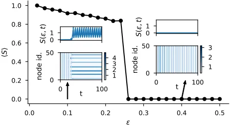
we introduce the macroscopic indicator
S(ǫ, t) = 1
Nkx(t)−x(¯ t)k
2, (22)
where ¯x(t) = (¯x, . . . ,x,¯ y, . . . ,¯ y¯). S(ǫ, t) enables us to quantify the, time-dependent, cumulative deviation be-tween individual oscillators trajectories, and the homo-geneous synchronized solution. S(ǫ, t) will rapidly con-verge to zero, if the synchronous state is stable. Con-versely, it will take non zero, positive values, when the imposed perturbation destroys the initial synchrony. To favor an immediate reading of the output quantities, we set to measure hSi, the average of S(ǫ, t), on one cycle Ts. In formulae, hSi =Ts−1
Rt+Ts
t S(ǫ, u) du, wheret is
larger than the typical relaxation time (transient). In Fig.2, main panel, hSiis plotted against ǫ, normalized to the value it takes in the limit ǫ → 0, for a choice of the parameter that corresponds to the dispersion relation depicted in Fig.1. A clear, almost abrupt, transition is seen, for ǫ∗ ≃ 0.25, in qualitative agreement with the above discussed scenario. Forǫ < ǫ∗, the oscillation are turned into a stationary stable pattern, as displayed in the annexed panel. By monitoringS(ǫ, t) for a choice of ǫbelow the critical threshold, one observes regular oscil-lations that can be traced back to the term ¯x in equa-tion (22). At variance, synchronous oscillations prove robust to external perturbation when ǫ > ǫ∗: the order parameterS(ǫ, t) is identically equal to zero, the two con-tributions in the argument of the sum on the right hand side of equation (22) canceling mutually.
To conclude the analysis, we will provide an approxi-mate theoretical estiapproxi-mate of the critical thresholdǫ. The proof of the partial averaging theorem, as outlined above, assumes an invertible change of coordinates. It is there-fore reasonable to quantifyǫ∗ by determining the range ǫfor which the invertibility condition is matched [29]. In formulae:
ǫ∗= min{ǫ >0 : det Γ(ǫ) = 0}. (23)
Using the block structure of ∂u/∂z=R0τ[L(t)− hLi] dt, one gets a more explicit form of the determinant
det(12N+ǫ∂u/∂z) =
det
1N +ǫDx
Z τ
0
[L(t)− hLi] dt
×det
1N +ǫDy
Z τ
0
[L(t)− hLi] dt
, (24)
which is zero if either of the determinants is zero. A straightforward manipulation yields, for the inspected network model, the following closed expression:
ǫ∗≃ 1 ΛN
12γ(1−γ)T min
1 Dx
, 1 Dy
, (25)
where ΛN
12 stands for the maximum eigenvalue (in ab-solute magnitude) of the operator (L1−L2), with L1
and L2 being the Laplacian matrices associated to the static networks as specified by the adjacency matricesA1 and A2. Performing the calculation returns ǫ∗ = 0.12, a coarse approximation of the exact critical value, as de-termined via direct numerical integration [38].
0 γTs Ts (1+γ)Ts 2Ts
A
(
t
) A11
2 3
45 6 A21 2 3
45 6 A11 2 3
45 6 A21 2 3 45 6 ⋯
(a)
1 2 3 4
5 6 1 2 3 4
5 6 time average ⟨A⟩
γ 1−γ
(b)
0⋯0 0⋯5 1⋯0 1⋯5 2⋯0 −⟩α
−2⋯0 −1⋯5 −1⋯0 −0⋯5 0⋯0 0⋯5
ma
⟨
R
e
μ
(
α
)
(c) (d)
0 1 2 3
FIG. 1. Instability in time-varying networks. (a) Dynamics
ofA(t), as obtained by alternating two static networks with
adjacency matrices A1 and A2 (see main text for a detail
account of the imposed couplings), over a cycle of time
du-rationTs. Each network in this illustrative example is made
ofN = 6 nodes. (b) The associated time-averaged network
hAi=γA1+(1−γ)A2. (c) Dispersion relation (max (Reµα)
against−Λα) obtained by assuming (i) the averaged network
hAi(red circles), (ii) each static network (black stars) and (iii)
the continuous support case (black curve). The networks are generated according to the procedure discussed in the main
body of the paper, but assuming nowN= 50. Other
parame-ters are set tob= 4.5,c= 2.5,Dx= 2,Dy= 20,Ts= 1, and
γ= 0.3. (d) Asymptotic, stationary stable patterns, obtained
forǫ= 0.1< ǫ∗. Shades of grey represent the value of thex
variable.
Finally, we shall inspect how the oscillation death phe-nomenon is influenced by the strength of the imposed coupling, here exemplified by the constantDy, which we
modulate when freezingDxto a nominal value. In Fig.3
different attractors, and their associated stability, are de-picted, for species x, for distinct choices of the control parameterDy. Here, the Brussellator model is assumed
[image:5.612.321.560.124.279.2]man-0.0 0.1 0.2 0.3 0.4 0.5
ε
0.0 0.2 0.4 0.6 0.8 1.0
⟨S
⟩
0 100
t
0 50
no
de
⟨id
.
1 2 3 4 0
1
S⟩
ε,
t)
0 t 100 0
50
no
de
⟨id
.
1 2 3 0
1
S⟩
ε,
t)
FIG. 2. Critical threshold ǫ∗. Average pattern amplitude,
hSi, as a function ofǫ, normalized to the amplitude of the
pat-tern referred to the averaged networkhAi=γA1+ (1−γ)A2
(as formally recovered in the limit ǫ → 0). Here, N = 50
nodes. Other parameters are set tob= 4.5,c= 2.5,Dx= 2,
Dy= 20, andγ= 0.3. (Insets) Dynamics ofx, on each node,
over time. Shades of blue represent the value of x. (Left)
for ǫ = 0.1, the synchronous solution is unstable. After a
transient time, oscillation death is seen, and a heterogeneous
pattern develops. (Right) for ǫ = 0.4, the synchronous
so-lution is stable. S(ǫ, t) is also plotted vs. time for the two
considered settings.
ifolds which delineate the boundaries of the associated basins of attractions are not displayed for graphic require-ments. Open (white) circles follow direct integration of model (1). In the simulations, ǫ is set to 0.1: the slight discrepancy between predicted and observed value ofDy
(at the onset of the desynchronization) stems from finite size corrections (the theory formally applies to the ideal-ized settingǫ→0). When synchrony is lost, the system evolves towards an asymptotic state that displays oscilla-tion death: each node is associated to a staoscilla-tionary stable density, which is correctly explained by resorting to the average model approximation (7). Increasing further the coupling strength Dy, results in a significant
complexi-fication of the phase space diagram, which considerably enrich the zoology of the emerging oscillation death pat-terns, as displayed in Fig.3above the supercritical pitch-fork bifurcations.
Summing up, we have here considered the synchronous dynamics of a collection of self-excitable oscillators, cou-pled via a generic graph. The plasticity of the underlying network of couplings, i.e. its inherent ability to adjust in time, may seed an instability which destroys synchrony. The system endowed with a time-varying network of
in-terlinked connections, behaves as its (partially) averaged analogue, provided the network dynamics is sufficiently fast. This result is formally established by resorting to an extended version of the celebrated averaging theorem, which allows for partial averages to be performed. In-terestingly, the network driven instability materializes in asymptotic, stationary stable patterns. These latter are to be regarded as a novel evidence for the oscillation death phenomenon.
10 20 30
Dy 0
1 2 3
x
10 20 30 0.4
0.6
FIG. 3. Phase diagram for the Brusselator model coupled via time dependent pairwise exchanges, as illustrated in the
caption of Fig. 1, with N = 6. The equilibrium solutions
relative to speciesxare plotted by varyingDy, at fixedDx=
2. The stability is computed for the average analogue (7) of
model (1). The horizontal (red, straight) lines refer to the
limit cycle: the maximum and minimum values as attained by the uncoupled oscillators, over one period, are respectively displayed. Black lines stand for the fixed points. Dashed lines refer to the unstable solutions, whereas solid lines implies stability. White circles are obtained from direct simulations
of model (1) withǫ= 0.1 and illustrate the oscillation death
phenomenon, as discussed in the main text. The panel on the right is a zoom of the lower portion of the main plot. The shaded regions are drawn to guide the reader’s eye across the different regimes: synchronization, oscillation death with 3-fixed point pattern, and oscillation death with 6-3-fixed point pattern correspond to the region in white, light gray, and dark gray, respectively. Notice that we chose to display a partial subset of the complete phase diagram. All stable manifolds are plotted. A limited subset of the existing unstable branches is instead shown for graphic requirements.
This work has been funded by the EU as Horizon 2020 research and innovation programme under the Marie Sk lodowska-Curie grant agreement No 642563.
[1] G. Nicolis and I. Prigogine,Self-organization in nonequi-librium systems (Wiley, New York, 1977).
[2] Y. Kuramoto, Chemical oscillations, waves, and turbu-lence(Springer-Verlag, Tokyo, 1984).
[3] A. Goldbeter, Biochemical Oscillations and Cellu-lar Rhythms (Cambridge University Press, Cambridge,
1997).
[4] A. Pikovsky, M. Rosenblum, and J. Kurths, Synchroniza-tion: A Universal Concept in Nonlinear Sciences, Vol. 12 (Cambridge University Press, Cambridge, 2003).
[image:6.612.58.293.59.189.2] [image:6.612.326.556.163.299.2][6] Y. F. Suprunenko, P. T. Clemson, and A. Stefanovska, Phys. Rev. Lett.111, 024101 (2013).
[7] M. Lucas, J. Newman, and A. Stefanovska, “Sta-bilisation of dynamics of oscillatory systems by non-autonomous perturbation,” (2017), submitted to Phys. Rev. E.
[8] M. Barahona and L. M. Pecora, Phys. Rev. Lett. 89, 054101 (2002).
[9] A. Arenas, A. Daz-Guilera, J. Kurths, Y. Moreno, and C. Zhou,Phys. Rep.469, 93 (2008).
[10] S. H. Strogatz and R. E. Mirollo,J. Stat. Phys.63, 613 (1991).
[11] H. Kori and A. S. Mikhailov,Phys. Rev. E 74, 066115 (2006).
[12] E. Ott and T. M. Antonsen,Chaos18, 037113 (2008). [13] S. Petkoski and A. Stefanovska,Phys. Rev. E86, 046212
(2012).
[14] G. Lancaster, Y. F. Suprunenko, K. Jenkins, and A. Ste-fanovska,Sci. Rep.6, 29584 (2016).
[15] B. Pietras and A. Daffertshofer,Chaos26, 103101 (2016).
[16] M. G. Earl and S. H. Strogatz,Phys. Rev. E67, 036204 (2003).
[17] Z. Hou and H. Xin,Phys. Rev. E68, 055103 (2003).
[18] W. Zou, X.-G. Wang, Q. Zhao, and M. Zhan, Front. Phys. China4, 97 (2009).
[19] H. Nakao and A. S. Mikhailov,Nat. Phys.6, 544 (2010).
[20] J. D. Challenger, R. Burioni, and D. Fanelli,Phys. Rev. E92, 022818 (2015).
[21] A. Koseska, E. Volkov, and J. Kurths,Phys. Rep.531, 173 (2013).
[22] M.-Y. Kim, R. Roy, J. L. Aron, T. W. Carr, and I. B. Schwartz,Phys. Rev. Lett.94, 088101 (2005).
[23] P. Kumar, A. Prasad, and R. Ghosh, J. Phys. B 41, 135402 (2008).
[24] M. Asllani and T. Carletti,arXiv:1703.06096 (2017).
[25] R. Arumugam, P. S. Dutta, and T. Banerjee,Phys. Rev. E94, 022206 (2016).
[26] P. Holme and J. Saramki,Phys. Rep.519, 97 (2012).
[27] P. Holme,Eur. Phys. J. Bs88, 234 (2015).
[28] N. Masuda and R. Lambiotte,A Guidance to Temporal Networks (World Scientific, Singapore, 2016).
[29] J. Petit, B. Lauwens, D. Fanelli, and T. Carletti,Phys. Rev. Lett.119, 148301 (2017).
[30] A. M. Turing,Philos. Trans. Royal Soc. B237, 37 (1952).
[31] Y. Sugitani, K. Konishi, and N. Hara, inNonlinear Dy-namics of Electronic Systems: 22nd International Con-ference, NDES 2014, Albena, Bulgaria, July 4-6, 2014. Proceedings, Vol. 438 (Springer, 2014) p. 219.
[32] P. E. Kloeden and M. Rasmussen,Nonautonomous Dy-namical Systems(American Mathematical Society, Prov-idence, 2011).
[33] F. Verhulst,Nonlinear differential equations and dynam-ical systems (Springer Science & Business Media, 1990).
[34] The diagonalizability of the Laplacian matrix is a mini-mal requirement for the analytical treatment to hold true. This condition is trivially met when the network of cou-plings is assumed symmetric, as in the example worked out in the following.
[35] M. Asllani, J. D. Challenger, F. S. Pavone, L. Sacconi, and D. Fanelli,Nat. Commun.5, 4517 (2014).
[36] M. Asllani, D. M. Busiello, T. Carletti, D. Fanelli, and G. Planchon,Phys. Rev. E90, 042814 (2014).
[37] This condition needs to be relaxed when dealing with di-rected graphs. The general philosophy of the calculation remains however unchanged, at the price of some techni-cal complication as discussed in [35].
[38] As an alternative for computing ǫ∗, assume T and ǫTs
are commensurable (if not, adjust the value of ǫ corre-spondigly) and define the common period for the reaction and diffusion parts,
Tc= LCM(T, ǫTs).
Compute the Floquet multipliers for the 2N×2Nsystem which is periodic with period Tc. Repeating the above procedure for decreasing values ofǫ(and making sureT