Implementing Monte Carlo Tests with P value Buckets

Implementing Monte Carlo Tests with P-value Buckets

Axel Gandy, Georg Hahn and Dong Ding Department of Mathematics, Imperial College London

Abstract

Software packages usually report the results of statistical tests using p-values. Users often interpret these by comparing them to standard thresholds, e.g. 0.1%, 1% and 5%, which is sometimes reinforced by a star rating (***, **, *). In this article, we consider an arbitrary statistical test whose p-valuepis not available explicitly, but can be approx-imated by Monte Carlo samples, e.g. by bootstrap or permutation tests. The standard implementation of such tests usually draws a fixed number of samples to approximate p. However, the probability that the exact and the approximated p-value lie on different sides of a threshold (the resampling risk) can be high, particularly for p-values close to a threshold. We present a method to overcome this. We consider a finite set of user-specified intervals which cover [0,1] and which can be overlapping. We call these p-value buckets. We present algorithms that, with arbitrarily high probability, return a p-value bucket containingp. We prove that for both a bounded resampling risk and a finite run-time, overlapping buckets need to be employed, and that our methods both bound the resampling risk and guarantee a finite runtime for such overlapping buckets. To interpret decisions with overlapping buckets, we propose an extension of the star rating system. We demonstrate that our methods are suitable for use in standard software, including for low p-values occurring in multiple testing settings, and that they can be computationally more efficient than standard implementations.

Keywords: Algorithms, Bootstrap/resampling, Hypothesis Testing, Sampling

1

Introduction

Software packages usually report the significance of statistical tests using p-values. Most users will base further steps of their analyses on where those p-values lie with respect to certain thresholds. To facilitate this, many tests in statistical software such as R (R Development Core Team, 2008), SAS (SAS Institute Inc., 2011) or SPSS (IBM Corp., 2013) translate the significance to a star rating system, in which typically p ∈(0.01,0.05] is denoted by *,

p∈(0.001,0.01] is denoted by ** andp≤0.001 is denoted by ***.

In this article, we consider a statistical test whose p-valuepcan only be approximated by sequentially drawn Monte Carlo samples. Among others, this scenario arises in bootstrap or permutation tests, see e.g. Lourenco and Pires (2014); Mart´ınez-Camblor (2014); Liu et al. (2013); Wu et al. (2013); Asomaning and Archer (2012); Dazard and Rao (2012).

Standard implementations of Monte Carlo tests in software packages usually take a fixed number of samples and estimatep as the proportion of exceedances over the observed value of the test statistic. Examples of this include the computation of a bootstrap p-value inside the function chisq.test in R or the function t-test in SPSS. However, there is no control of theresampling risk, the probability that the exact and the approximated p-value lie on two opposite sides of a testing threshold (usually 0.1%, 1% or 5%).

Sequential methods to approximate p-values have been studied in the literature. Early works provided ad hoc attempts to reduce the computational effort without focusing on a specific error criterion (Besag and Clifford, 1991; Silva et al., 2009).

Further developments aimed at a uniform bound on the resampling risk for a single threshold (Davidson and MacKinnon, 2000; Andrews and Buchinsky, 2000, 2001; Gandy, 2009). Gandy (2009) shows that such a uniform bound necessarily results in an infinte running time.

There are also approaches that aim to bound an integrated resampling risk for a single threshold (Fay and Follmann, 2002; Kim, 2010; Silva and Assun¸c˜ao, 2013). Such an error criterion is weaker that a uniform bound on the resampling risk and can be achieved with finite effort.

In this article, we present algorithms that work with multiple thresholds, aim for uniform bounds on the error and, under conditions, have finite running time. We first generalize testing thresholds to a finite set of user-specified intervals (called “p-value buckets”) which cover [0,1] and which can be overlapping. Our algorithms return one of those p-value buckets which is guaranteed to contain the unknown (true)p up to a uniformly bounded error.

We prove that methods achieving both a finite runtime and a bounded resampling risk need to operate on overlapping p-value buckets. In order to report decisions computed with overlapping buckets, we propose to use an extension of the classical star rating system (*, **, ***) used to indicate the significance of a hypothesis.

Our methods rely on the computation of a confidence sequence forp. We present two ap-proaches to compute such a confidence sequence, prove that both apap-proaches indeed bound the resampling risk and achieve a finite runtime for overlapping buckets. We compare both approaches in a simulation section and demonstrate that they achieve a competitive compu-tational effort which is close to a theoretical lower bound on the effort we derive.

The article is structured as follows. Section 2 introduces the mathematical setting of our article (Section 2.1), the rationale behind overlapping p-value buckets (Section 2.2), our proposed extension of the traditional star rating system (Section 2.3) and a general algorithm to compute a decision for pwith respect to a set of p-value buckets (Section 2.4). The general algorithm relies on the construction of certain confidence sequences for p for which we present two approaches: one based on likelihood martingales (Robbins, 1970; Lai, 1976) in Section 3.1 and one based on theSimctest algorithm (Gandy, 2009) in Section 3.2. In Section 4 we first derive a theoretical lower bound on the expected effort (Section 4.1) and demonstrate that our methods achieve a computational effort which stays within a multiple of the optimal effort (Sections 4.2, 4.3). An application to multiple testing is considered in Section 4.4. The article concludes with a discussion in Section 5. All proofs can be found in Appendix A. The Supplementary Material includes R-code to implement the algorithms as well as to reproduce all figures and tables.

2

General algorithm

2.1 Setting

We consider one hypothesis H0 which we would like to test with a given statistical test.

Let T denote the test statistic and let t be the evaluation of T on some given data. For simplicity, we assume that H0 should be rejected for large values of t. In this case the

p-value is commonly defined as the probability of observing a statistic at least as extreme as

t, i.e.

p=P(T ≥t), (1)

whereP is a probability measure under the null hypothesis.

Bucket [0,0.1%] (0.1%,1%] (1%,5%] (5%,1]

Code *** ** *

Bucket (0.05%,0.2%] (0.8%,1.2%] (4.5%,5.5%]

Code **∼ *∼ ∼

Table 1: Extended star rating system for the p-value buckets J∗.

test statisticT on them. Comparing the result to the observed realization of T then allows to approximate the p-value as ˆp = Pn(T ≥t), where Pn is the estimated null-distribution based onnsamples (for instance, using bootstrap tests). The exceedances over the observed realization ofT can equivalently be modeled using a stream of independent random variables

Xi,i∈N, having a Bernoulli(p) distribution.

LetJ be a set of sub-intervals of [0,1] of positive length that cover [0,1], i.e. S

J∈J J =

[0,1]. We call any suchJ a set of p-value buckets. For example,

J =J0 :={[0,10−3],(10−3,0.01],(0.01,0.05],(0.05,1]} (2)

is a set of p-value buckets. Finding a bucketI ∈ J0_{such thatp∈I is equivalent to deciding}

wherep lies in relation to the traditional levels 0.001, 0.01 and 0.05.

The goal of our algorithms is to find a bucket I ∈ J containing p. A natural error criterion is the risk of a wrong decision Pp(p /∈ I), which we call the resampling risk. Our methods bound the resampling risk uniformly inp at a given ∈(0,1), i.e.

Pp(p /∈I)≤for all p∈[0,1]. (3)

We will show that there is no algorithm achieving this forJ0 _{with finite expected effort –}

for finite effort we needoverlapping p-value buckets, which we discuss in the next section.

2.2 Overlapping buckets

We say that the bucketsJ are overlapping if any p∈(0,1) is contained in the interior of a

J ∈ J. For instance, the bucketsJ0 _{in (2) are not overlapping, whereas the buckets}

J∗=J0∪

(5·10−4,2·10−3],(0.008,0.012],(0.045,0.055] ,

employed in the remainder of this article, are overlapping.

We letτ be the random effort of an algorithm, defined as the number of exceedance indi-catorsXi used. The following theorem shows that overlapping buckets are both a necessary and sufficient prerequisite for a finite time algorithm satisfying (3) to exist.

Theorem 1. The following statements are equivalent:

1. There exists an algorithm satisfying (3)with Ep[τ]<∞ for all p∈[0,1].

2. The p-value buckets J are overlapping.

3. There exists an algorithm satisfying (3)with τ < C for some deterministic C >0.

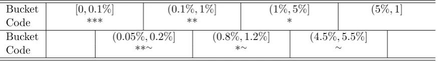
2.3 Extended Star Rating System

Figure 1: Left: Non-stopping region (gray) to decidep with respect to Je (corresponding to a 5% threshold). Right: Non-stopping region for the overlapping bucketsJe∪ {(0.03,0.07]}.

manual of the American Psychological Association (American Psychological Association, 2010, page 139), is the de facto standard for reporting significance. As we have seen in Theorem 1, it is impossible to produce such a star rating for Monte Carlo tests with finite effort, but it is possible to report results with overlapping buckets with finite effort.

We propose to extend the star rating system to overlapping buckets as described in Table 1, using the p-value buckets J∗ as example. If the algorithm gives a clear decision with respect to the classical thresholds, we report the classical star rating. Otherwise, i.e. if the reported bucket I equals (0.05%,0.2%], (0.8%,1.2%] or (4.5%,5.5%], we propose to report significance with respect to the smallest classical threshold larger than maxI and to indicate the possibility of a higher significance with a tilde symbol.

For instance, suppose an algorithm returns the bucket I = (0.05%,0.2%] for p upon stopping. Since in this case a decision with respect to all classical thresholds larger than maxI = 0.2% is available, we know that p ≤ 1% and can safely report a ** significance. However, as p could either be smaller or larger than the next smaller classical threshold 0.1%∈J, we report **∼ to indicate the possibility of a higher significance.

2.4 The general construction

We suppose that for each n ∈ _N, we can compute a confidence interval In for p based on

X1, . . . , Xn such that the joint coverage probability of the sequence In, n ∈ N, is at least 1−, where >0 is the desired uniform bound on the resampling risk, i.e. we require

Pp(p∈In ∀n∈N)≥1− for all p∈[0,1]. (4)

In Sections 3.1 and 3.2 we consider two constructions satisfying (4). For a given setJ of p-value buckets, we define the stopping time

τJ = inf{n∈N:∃I ∈ J :In⊆I} (5) which denotes the minimal number of samplesnneeded until a confidence intervalIn is fully contained in a bucket I ∈ J. The result of our algorithm is this bucket I if τJ < ∞. If

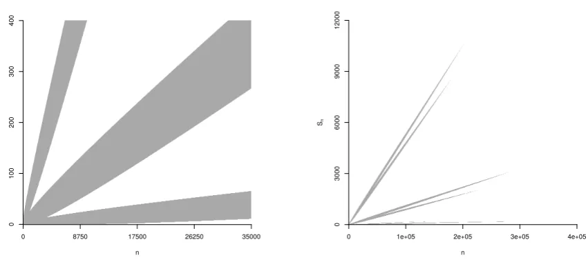
Figure 2: Non-stopping region forJ0 _{(left) andJ}∗ _(right).

The random intervalI constructed in this way satisfies the uniform bound on the resam-pling risk (3) due to the strong law of large numbers and due to (4).

If τJ is bounded, meaning if there existsN ∈N such thatτJ < N, we can relax (4) to

Pp(p∈In∀n < N)≥1− for all p∈[0,1]. (6)

Example 1. Suppose we are solely interested in the 5% threshold. Testing at 5% corresponds to the two classical bucketsJe={[0,0.05],(0.05,1]}. Using the approach of Section 3.2 with

= 10−3 to compute a confidence sequence forp, we arrive at the non-stopping region (gray) displayed in Figure 1 (left).

Sampling progresses until the sampling path (n, Sn)hits either (lower or upper) boundary

of the non-stopping region. As displayed in Figure 1 (left), we report the interval [0,0.05] ((0.05,1]) upon hitting the lower (upper) boundary first.

Adding the bucket (0.03,0.07] to Je results in overlapping buckets with a finite non-stopping region displayed in Figure 1 (right). In Figure 1 (right), the sample path can leave the non-stopping region in three ways: Either to the top via the former upper boundary of Figure 1 (left), in which case we report the classic interval (0.05,1], to the bottom via the former lower boundary corresponding to the bucket [0,0.05], or to the middle corresponding to the added bucket (0.03,0.07].

Example 2. Similarly to Example 1, Figure 2 shows the non-stopping region forJ0 _andJ∗_.

Again, the stopping region is infinite for the non-overlappingJ0 _{and finite forJ}∗ _consisting

of overlapping p-value buckets.

How likely is it to observe the different decisions possible when testing withJ∗? Figure 3 shows the probability of obtaining each decision in the extended star rating system forJ∗ as a function ofp. These probabilities are computed as follows: For a givenp, we iteratively (over

n) compute the distribution of Sn conditional on not stopping. This allows us to compute

the probability of stopping and the resulting decision.

Figure 3: Probabilities of observing each possible decision with J∗ as a function ofp.

3

Construction of Confidence Sequences

We now present two approaches to computing confidences sequences and show that, for overlapping buckets, the resulting stopping times are bounded.

3.1 The Robbins-Lai approach

Confidence sequences can be constructed from likelihood martingale inequalities (Robbins, 1970; Lai, 1976). To be precise, Robbins (1970) proves that the following inequality

Pp

∃n∈_N:b(n, p, Sn)≤

n+ 1

≤ (7)

holds true for allp∈(0,1) and ∈(0,1), whereb(n, p, x) = n_xpx(1−p)n−x. The statement (7) is trivially true for p ∈ {0,1}. Therefore, In ={p ∈[0,1] : (n+ 1)b(n, p, Sn) > } is a sequence of confidence sets forp with the desired coverage probability of 1−.

Lai (1976) further shows that In are intervals. Indeed, if 0 < Sn < n we have In = (gn(Sn), fn(Sn)), where gn(x)< fn(x) are the two distinct roots of (n+ 1)b(n, p, x) =. In the caseSn= 0, the equation (n+1)b(n, p, x) =has only one rootrn, leading toIn= [0, rn). Likewise for the caseSn=n, which leads toIn= (rn,1].

For overlapping bucketsJ, the stopping timeτJ can always be bounded by a

determinis-tic positive constant. Indeed, the following two lemmas show that the length ofInuniformly goes to zero and, moreover, that once an interval is below a certain length, it is guaranteed to be contained in one of the buckets, ensuring that the general algorithm stops.

Lemma 1. Let n∈_Nand|In|be the length of the interval In. Then |In| ≤

₂

nlog n+1

1/2

.

Lemma 2. If J is an overlapping set of p-value buckets then there exists c >0 s.t. for all intervals I ⊆[0,1]with length less than c there exists J ∈ J such that I ⊆J.

3.2 The Simctest approach

Gandy (2009) constructed stopping boundaries to compute a decision for a p-value with respect to a single thresholdα∈[0,1]. We revisit this method before showing how it can be extended to p-value buckets.

Before observing Monte Carlo samples, two integer sequences (Li)i∈Nand (Ui)i∈Nserving

as lower and upper stopping boundaries are computed. The algorithm then proceeds to draw samples (Xi)i∈_N until the trajectory (n, Sn) hits either boundary. The stopping time for this method is thusτ = inf{k∈N:Sk≥Uk orSk≤Lk}.

The two boundaries (Li)i∈Nand (Ui)i∈N are a function of both the thresholdαand some

bound on the resampling risk ρ. They are computed recursively in such a way that, given

p≤α(p > α), the probability of hitting the upper (lower) boundary is less than ρ. Starting withU1 = 2,L1 =−1, the two sequences are recursively defined as

Un= min{j∈N:Pα(τ ≥n, Sn≥j) +Pα(τ < n, Sτ ≥Uτ)≤n},

Ln= max{j ∈Z:Pα(τ ≥n, Sn≤j) +Pα(τ < n, Sτ ≤Lτ)≤n}, (8)

where (n)n∈_N is a non-decreasing sequence satisfying n→ρ asn→ ∞and 0≤n ≤ρ. It controls how the overall errorρis spent over all iterations of the algorithm (called aspending sequence in Gandy (2009)). In the remaining sections of this article we use

n=ρ

n

n+k (9)

withk= 1000, which is thedefault spending sequence suggested in Gandy (2009).

The aforementioned method has a finite expected stopping time (for p 6= α) and the probability of hitting thewrong boundary (leading to a decision not equal to the one obtained based on the unknownp) is bounded byρ(under the conditionsρ≤1/4 and log(n−n−1) =

o(n) as n→ ∞, see (Gandy, 2009, Theorem 1)). Thus, upon stopping we define I = [0, α] in case of hitting the lower boundary (Sτ ≤Lτ) andI = (α,1] in case of hitting the upper boundary (Sτ ≥Uτ). By construction, the interval I has a coverage probability of 1−ρ.

To extend the approach of Gandy (2009) to multiple thresholds we proceed as follows. We first define the set of boundaries of the intervals inJ that are in the interior of [0,1]:

AJ :={minJ, maxJ : J ∈ J } \ {0,1},

where minJ (maxJ) denote the lower (upper) limit of the intervalJ, respectively. Then we construct the above stopping boundaries for eachα ∈AJ, denoted asLn,α and Un,α, using the sameρ.

We define corresponding stopping times σα = inf{k ∈ N : Sk ≥ Uk,α orSk ≤ Lk,α} (based on the same sequenceXj, j∈N, see Section 2.1). We then define

In,α=



 

 

[0,1] ifn < σα,

[0, α) ifn≥σα, Sσα ≤Lσα,α,

(α,1] ifn≥σα, Sσα ≥Uσα,α,

and letIn=T_α∈AJ In,α.

The following theorem shows that In has the desired joint coverage probability given in (4) or (6) when settingρ=/2.

Theorem 2. Let N ∈ N∪ {∞}. Suppose that Un,α ≤ Un,α0 and L_n,α ≤ L_n,α0 for all

α, α0 ∈AJ, α < α0, and n < N (computed as in (8) with overall error ρ for each α ∈AJ).

Then for all p∈[0,1],

Allowing N <∞ is useful for stopping boundaries constructed to yield a finite runtime (see (6)).

The condition on the monotonicity of the boundaries (Un,α ≤Un,α0 and L_n,α ≤L_n,α0 for

all n ∈ _N and α, α0 ∈ J with α < α0) can be checked for a fixed spending sequence n in two ways: For finite N, the two inequalities can be checked manually after constructing the boundaries. ForN =∞, the following lemma shows that under conditions, the monotonicity of the boundaries holds true for all n≥n0, wheren0 ∈N can be computed as a solution to inequality (15), given in the proof of Lemma 3 in Appendix A. For n < n0, the inequalities

again have to be checked manually.

Lemma 3. Suppose ρ ≤ 1/4 and log(n−n−1) = o(n) as n → ∞. Let α, α0 ∈ AJ with

α < α0. Then there exists n0 ∈Nsuch that for all n≥n0,

Ln,α ≤Ln,α0, U_n,α ≤U_n,α0.

The condition on the spending sequence in Lemma 3 is identical to the condition im-posed in Theorem 1 of Gandy (2009) and is satisfied by the default spending sequence (9). Therefore, our default spending sequence (9) with the p-value buckets used in this article (J0 _{and J}∗_{) satisfies the boundary conditions of Theorem 2.}

The following theorem shows that for overlapping buckets the algorithm has a bounded stopping time.

Theorem 3. Suppose the conditions of Theorem 2 and Lemma 3 hold true withN =∞. If J is a finite set of overlapping p-value buckets then the general construction of Section 2.4 has a bounded stopping time τJ, i.e. there exists c <∞ s.t. τJ ≤c.

4

Computational effort

This section investigates the expected computational effort of the algorithm of Section 2.4. We start by deriving a theoretical lower bound on the expected effort in Section 4.1. We then compare both the Simctest and Robbins-Lai approach of Section 3 in terms of their expected effort as a function of p (Section 4.2). Integrating this effort for certain p-value distributions of practical interest allows to compare both approaches in practical situations (Section 4.3). Section 4.4 shows that the algorithm can be used for small p-values arising in multiple testing settings.

4.1 Lower bounds on the expected effort

In this section we construct lower bounds on the expected number of steps of sequential procedures satisfying (3). The key idea is to consider hypothesis tests implied by (3) and then to use the lower bounds for the expected effort of sequential tests (Wald, 1945, eq. (4.80)).

We suppose that I is the (random) bucket reported by a sequential procedure that re-spects (3). Let ˜p∈[0,1]. We give a basic and an improved lower bound on Ep˜[τ].

First, let ˜J = S

J∈J,p˜∈JJ be the union of all buckets that ˜p is contained in. For any

q∈[0,1]\I˜, we can consider the hypothesesH0:p= ˜p againstH1:p=q and the test that

rejects H0 iff p /∈ I. By (3), the type I error of such a test is at most . Also, the type II

error is at most, as P_q(p∈I)≤ P_q(q /∈I)≤. Hence,Ep˜[τ] is bounded from below by the

lower bound in (Wald, 1945, eq. (4.80)), which we calla(q). Thus we get

Ep˜[τ]≥max

q /∈J˜

a(q). (10)

Figure 4: Basic (gray) and improved (black) lower bounds on the effortEp[τ] for the buckets

J∗.

The bound (10) can be improved if the number of elements of J containing ˜p is exactly two, say J1 and J2. Suppose that for a given sequential procedure, η = Pp˜(I1). Let q1 ∈

[0,1]\J1. Consider the hypotheses H0 :p= ˜p and H1 :p= q1 and the corresponding test

that rejectsH0 iff I 6=J1. This test has type I error 1−η and type II error . Again, using

(Wald, 1945, eq. (4.80)) we get a lower bound onEp˜[τ], which we callb1(q, η). Similarly, for

any q2 ∈[0,1]\J2, we can test the hypotheses H0 :p = ˜p and H1 :p =q2 by rejectingH0

iffI 6=J2. This test has type I error of at most η+and type II error of at most . Again,

using (Wald, 1945, eq. (4.80)) we get a lower bound onEp˜[τ], which we call b2(q, η).

Asηis dependent on the specific procedure, we can get a universal lower bound onEp˜[τ]

by minimizing overη, thus

Ep˜[τ]≥max max

q /∈_J˜ a(q),ηmin∈[0,1]max

max q /∈J1

b1(q, η),max

q /∈J2

b2(q, η)

!

. (11)

The maxima in (11) can be evaluated by looking at the boundary points of ˜J, J1 and

J2. The minimum can be bounded from below by looking at a grid of values for η and

conservatively replacingb2(q, η) byb2(q, η+δ), whereδ is the grid width.

Figure 4 gives an example of both the basic and the improved lower bound on Ep˜[τ] for

the buckets J∗. The improved bound is much higher (and thus better) in the areas where there are overlapping buckets.

4.2 Expected effort for (non-)overlapping buckets

This section investigates both the non-overlapping p-value bucketsJ as well as the overlap-ping bucketsJ∗ _{with respect to the implied expected effort as a function ofp.}

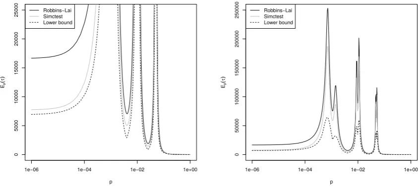
Using the non-stopping regions depicted in Figure 2, Figure 5 shows the expected effort (measured in terms of the number of samples drawn) to compute a decision with respect to J (left) and J∗ _{as a function of p ∈ [10}−6_{,1]. For any given p, the expected effort is}

Figure 5: Expected effort to compute a decision with respect to J (left) and J∗ _{(right) as}

a function of p. Both Simctest and Robbins-Lai are used to compute confidence sequences. Lower bound on the effort given as dashed line.

stopped up to time n. Using this distribution, we work out the probability of stopping at stepn and add the appropriate contribution to the overall effort.

The effort diverges as p approaches any of the thresholds in J. For J∗ _{the effort stays}

finite even in the case that p coincides with one of the thresholds (Figure 5, right). The effort is maximal in a neighborhood around each threshold, while in-between thresholds, the effort slightly decreases. For p-values larger than the maximal threshold in J∗, the effort decreases to zero. The effort for Simctest seems to be uniformly smaller than the one for Robbins-Lai for bothJ and J∗.

Figure 5 also shows the lower bound (dashed line) on the effort derived in Section 4.1. In connection with Simctest, the effort of our algorithm of Section 2.4 differs from the theoretical lower bound by roughly a factor of three.

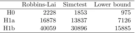
4.3 Expected effort for three specific p-value distributions

The expected effort of the proposed methods for repeated use can be obtained by integrating the expected effort for fixedp (Figure 5, right) with respect to certain p-value distributions. Here, we consider using the overlapping bucketsJ∗ with three different p-value distribu-tions. These are a uniform distribution in the interval [0,1] (H0), as well as two alternatives

given by the density 1₂+ 10I(x≤0.05) (H1a) and by a Beta(0.5,25) distribution (H1b), where I denotes the indicator function.

Robbins-Lai Simctest Lower bound

H0 2228 1853 975

H1a 16878 13837 7126

H1b 40059 30896 15885

Table 2: Expected (integrated) effort for both Robbins-Lai and Simctest applied toJ∗_.

Ex-pectations are taken over three different p-value distributions: a uniformU[0,1] distribution (H0) and two mixture distributions H1a and H1b.

4.4 Application to multiple testing

We consider the applicability of our algorithm of Section 2.4 to the (lower) testing thresholds occurring in multiple testing scenarios. In the following example, we demonstrate that our algorithm is well suited as a screening procedure for the most significant hypotheses: Even for small threshold values, it is capable of detecting more rejections than a na¨ıve sampling procedure that uses an equal number of samples.

We assume we want to test n = 104 hypotheses using the Bonferroni (1936) procedure to correct for multiplicity. In order to be able to compute numbers of false classifications, we assignnA= 100 hypotheses to the alternative, the remainingn−nA= 9900 hypotheses are from the null. The p-values of the alternative are then set to 1−F(X), where F is the cumulative distribution function of a Student’s t-distribution with 100 degrees of freedom and X is a random variable sampled from a t-distribution with 100 degrees of freedom and noncentrality parameter uniformly chosen in [2,6]. The p-values of the null are sampled from a uniform distribution in [0,1].

We apply our algorithm from Section 2.4 with = 10−3 and confidence sequences com-puted with the Simctest approach (Section 3.2). To speed up the Monte Carlo sampling, we sample in batches of geometrically increasing size aib in each iteration i, where b = 10 and a= 1.1. Likewise, both the stopping boundaries and the stopping condition (hitting of either boundary) in Simctest are updated (checked) in batches of the same size.

In order to screen hypotheses, we aim to group them by the order of magnitude of their p-values. For this we employ the overlapping buckets

Js=0,10−7 ∪

10i−2,10i:i=−6, . . . ,0

which group the p-values in buckets spanning two orders of magnitude each (and0,10−7). We now report the results from a single run of this setup. Our algorithm draws N = 3.2·105 samples per hypothesis. Of the 104 hypotheses, 28 are correctly allocated to the two lowest buckets. As expected, the p-values from the null are all allocated to larger buckets (covering values from 10−4 onwards).

An alternative approach would be to draw an equal number ofN samples per hypothesis and to compute a p-value using a pseudo-count (Davison and Hinkley, 1997). Due to this pseudo-count, this na¨ıve approach is incapable of observing p-values below N−1 = 3.125·

10−6, and in particular incapable of observing any p-values in the lower bucket.

5

Discussion

In this article we investigate methods capable of computing a decision for a single hypothesis

H0 with unknown p-value p (approximated via Monte Carlo sampling) that achieve both

In order to report decisions when testing with overlapping buckets, we propose to use an extension of the traditional star rating system used to report the significance of a hypothesis. Our algorithms rely on the computation of a confidence sequence for the unknownp. We give two constructions of such confidence sequences (Section 3), prove that both approaches indeed satisfy the bound on the resampling risk and yield a finite runtime for overlapping buckets. We (empirically) demonstrate that our methods achieve a competitive computa-tional effort that is close to a theoretical lower bound on the effort (Section 4).

The choice of (overlapping) p-value buckets we employ in our article is arbitrary. However, a variety of (heuristic) techniques can be used to obtain overlapping buckets from traditional thresholdsT ={t0, . . . , tm}. These include:

1. The bucket overlapping each threshold t ∈ T can be chosen as a fixed proportion

ρ∈(0,1), leading to the interval [ρt, ρ−1t].

2. Since the length of a confidence interval for a binomial quantitypbehaves proportion-ally to pp(1−p) ∈ O √p as p → 0, a bucket around any t ∈ T can be chosen as

J := [t−ρ√t, t+ρ√t], where ρ >0 is such that 0∈/J.

3. The buckets can be chosen to match the precision of a na¨ıve sampling method which draws a fixed number of samplesn∈_Nper hypothesis. For this we compute alln+ 1 possible confidence intervals (one for each possibleSn∈ {0, . . . , n}) for each threshold

t∈ T and record all confidence intervals which cover t. The union of those intervals can then be used as a bucket for t.

The tuning parameterρ can be chosen, for instance, to minimize the maximal (worst case) effort for the resulting overlapping buckets.

The present article leaves scope for a variety of future research directions. For instance, how can overlapping p-value buckets be chosen to maximize the probability of obtaining a classical decision (*, ** or ***), subject to a suitable optimization criterion? How can the lower bound on the computational effort derived in Section 4.1 be improved? Which algorithm (possibly based on our generic algorithm in connection with Simctest) is capable of meeting the lower bound effort?

A

Proofs

Proof of Theorem 1. We prove a circular equivalence of the three statements.

(1.) ⇒ (2.): Suppose the buckets J are not overlapping. This implies that there exists

α∈(0,1) that is not contained in the interior of any J ∈ J.

Let I ∈ J be the (random) interval reported by an algorithm satisfying (3). Let n∈N such thatα−1/n≥0 andα+ 1/n≤1.

Consider the hypotheses H0 :p=α−1/nandH1 :p=α+ 1/nand the test that rejects

H0 iff α−1/n /∈I. As I cannot contain both α−1/n and α+ 1/n (otherwise α would be

in the interior of the intervalI) and because of (3), this test has type I and type II error of at most. Hence, by the lower bound on the expected number of steps of a sequential test given in (Wald, 1945, equation (4.81)) (see also (Gandy, 2009, section 3.1)), we have

Eα+1/n[τ]≥

log(₁₋) + (1−) log(1−)

(α+_n1) log(α_α+1₋₁/n_/n) + (1−α−_n1) log(1₁−₋α_α−₊₁1/n_/n).

(2.)⇒(3.): We construct an explicit (but not very efficient) algorithm for this.

Let a0 < a1 < . . . < ak be the set of boundaries of buckets in J, i.e. {a0, . . . , ak} =

{maxJ :J ∈ J } ∪ {minJ :J ∈ J }. Let ∆ = min{ai−ai−1 :i= 1, . . . , k} be the minimal

gap between those boundaries.

LetI(S, n) be the two-sided Clopper and Pearson (1934) confidence interval with coverage probability 1−forp whennis the number of samples andS is the number of exceedances. Let n ∈ _N be such that the length of all Clopper-Pearson intervals is less than ∆, i.e.

n= min{m∈_N:∀S∈ {0, . . . , m}:|I(S, m)|<∆}. This is well-defined as the length of the Clopper Pearson confidence intervalI(S, n) decreases to 0 uniformly inS asn→ ∞; see e.g. the proof of Condition 2 in Lemma 2 of Gandy and Hahn (2014) for this.

Consider the algorithm that takes n samples X1, . . . , Xn and then returns an arbitrary interval I ∈ J that satisfies I ⊇ I(Pn

i=1Xi, n) (to be definite, order all elements in J arbitrarily and return the first element satisfying the condition. Such anI always exists as the buckets are overlapping by (2.) and as|I(Pn

i=1Xi, n)|<∆, implying that it overlaps with at most one possible boundary. This algorithm satisfies (3) due to the coverage probability of 1−of the Clopper-Pearson interval.

(3.)⇒(1.): Since finite effort implies expected finite effort, (1.) follows immediately.

Proof of Lemma 1. If 0 ≤ p ≤ Sn

n −

₁

2nlog n+1

1/2

then, by Hoeffding’s inequality (Ho-effding, 1963),

b(n, p, Sn) =P(X =Sn)≤ P

X n −p≥

Sn

n −p

≤exp

−2(Sn−np)2

n

≤

n+ 1,

whereX∼Bin(n, p) is a binomial random variable. Hence,p /∈In. A similar argument can be made for Sn

n +

₁

2nlog n+1

1/2

≤p≤1. Thus,|In| ≤

₂

nlog n+1

1/2

.

Proof of Lemma 2. Suppose this is not true. Then for all n ∈ N there exists an interval

In ⊂[0,1] with 0 <|In|< _n1 s.t. ∀J ∈ J: In 6⊆J. Let an be the mid points ofIn. As (an) is a bounded sequence, there exists a convergent subsequence (ank). Let b= limk→∞ank.

If b∈(0,1) then, as J is overlapping, there exists >0 and J ∈ J : (b−, b+)⊆J. For large enough kwe have Ink ⊆(b−, b+), contradicting Ink 6⊆J.

Ifb= 0 then, asJ is a covering of [0,1] consisting of intervals of positive length there exists

>0 and J ∈ J s.t. [0, )⊆J. For large enoughkwe have Ink ⊆[0, ), again contradicting

Ink 6⊆J. Ifb= 1 a contradiction can be derived similarly.

Proof of Theorem 2. For a given threshold α∈AJ, let

EN_α ={Sτα ≥Uτα,α, τα< N}

be the event that the upper boundary is hit first before time N and likewise let

EN_α ={Sτα ≤Lτα,α, τα< N}

be the event that the lower boundary is hit first. Then, for all α, α0 ∈AJ with α < α0 the

following holds:

EN_α ⊇EN_α0 and EN_α ⊆EN_α0. (12)

Indeed, to see EN_α ⊇ EN_α0, we can argue as follows. On the event E

N

α0, as U_n,α ≤ U_n,α0

for all n ∈ _N, the trajectory (n, Sn) must hit the upper boundary Un,α of α no later than

τα0, henceτ_α ≤τ_α0 < N. It remains to prove that the trajectory does not first hit the lower

its upper boundary, it also hits the lower boundary of α0 (as Ln,α ≤ Ln,α0 for all n < N)

before timeτα0, thus contradicting being on the event EN_α0. Hence, we haveE

N α ⊇E

N α0. The

proof ofEN_α ⊆EN_α0 is similar.

Using this notation, for all p∈[0,1],

Pp(∃n < N :p /∈In)≤ Pp(∃n < N, α∈AJ :p /∈In,α)

=P_p



 [

α∈AJ:α≤p

EN_α ∪ [

α∈AJ:α≥p

EN_α



≤ Pp



 [

α∈AJ:α≤p

EN_α



+Pp



 [

α∈AJ:α≥p

EN_α



.

(13)

Ifp < minAJ then the first term is equal to 0. Otherwise, let α0 = max{α∈AJ :α≤p}.

Then, by (12),

P_p



 [

α∈AJ:α≤p

EN_α



=P_p EN_α0

≤ρ.

The second term on the right hand side of (13) can be dealt with similarly.

Proof of Lemma 3. By arguments in (Gandy, 2009, Proof of Theorem 1), we have

Un,α−nα

n ≤

∆n+ 1

n →0,

Ln,α0 −nα0

n ≥ −

∆n+ 1

n →0 (14)

as n→ ∞, where ∆n =

p

−nlog(n−n−1)/2. Since ∆n =o(n) there existsn0 ∈ N such that 2 ∆n n + 1 n

≤α0−α for all n≥n0. (15)

Splitting _n2 = _n1 +_n1 and multiplying by n yieldsnα+ ∆n+ 1≤nα0−∆n−1 from which

Un,α ≤Ln,α0 follows by (14).

By definition, we have Ln,α ≤ Un,α and Ln,α0 ≤ U_n,α0 for all n ∈ _N, thus implying

Ln,α ≤Ln,α0,U_n,α ≤U_n,α0 for all n≥n₀ as desired.

Proof of Theorem 3. By (14) and as ∆n=o(n) there exists n0∈Nsuch that

|{α∈AJ :σα> n0}| ≤1. (16)

We will show thatτJ ≤n0.

First, the assumption on the ordering of Ln and Un exclude the possibility of In0 =∅.

Second, (16) implies|In0 ∩AJ| ≤1.

If|In0∩AJ|= 1 then let α∈AJ be such thatα∈In0. AsJ is overlapping, there exist

J ∈ J such that α is in the interior of J. Hence, α cannot be a boundary of J, implying

In0 ⊆J due to |In0 ∩AJ|= 1, thus showing τJ ≤n0.

If |In0 ∩AJ|= 0 then let β be in the interior of In0. As J is overlapping, there exists

J ∈ J such thatβ ∈J. AsIn0 ∩AJ =∅ this impliesIn0 ⊆J, showing τJ ≤n0.

B

A simple stopping criterion for Robbins-Lai

The following describes a simple criterion to determine whether a confidence interval com-puted via Robbins-Lai (Section 3.1) is fully contained in a bucket. Let intervalInand bucket

J ∈ J as well asn,Sn and be as in Section 3.1. ThenIn⊆J if and only if

(n+ 1)b(n, Sn, p) = (n+ 1)

n Sn

forp∈ {minJ,maxJ}.

As (17) is also satisfied ifI andJ are simply disjoint, we verify that (n+ 1)b(n, Sn, p) is indeed increasing at minJ and decreasing at maxJ using the derivative of (n+ 1)b(n, Sn, p) with respect to p. This then proves that the two limits of bucket J are indeed not both smaller than minI or larger than maxI. We first apply a (monotonic) log transformation,

log [(n+ 1)b(n, Sn, p)] = log(n+ 1) + log

n Sn

+Snlogp+ (n−Sn) log(1−p),

and then take the derivative with respect top:

Sn

p −

n−Sn 1−p

(

≥0 p= minJ,

≤0 p= maxJ. (18)

If (17) and (18) are satisfied, thenIn⊆J.

References

American Psychological Association (2010). Publication manual of the American Psycholog-ical Association (6th ed.). American Psychological Association, Washington, DC.

Andrews, D. and Buchinsky, M. (2000). A three-step method for choosing the number of bootstrap repetitions. Econometrica, 68(1):23–51.

Andrews, D. and Buchinsky, M. (2001). Evaluation of a three-step method for choosing the number of bootstrap repetitions. J Econometrics, 103(1-2):345–386.

Asomaning, N. and Archer, K. (2012). High-throughput DNA methylation datasets for evaluating false discovery rate methodologies. Comput Stat Data An, 56(6):1748–1756.

Besag, J. and Clifford, P. (1991). Sequential Monte Carlo p-values. Biometrika, 78(2):301–4.

Bonferroni, C. (1936). Teoria statistica delle classi e calcolo delle probabilit`a. Pubblicazioni del R Istituto Superiore di Scienze Economiche e Commerciali di Firenze, 8:3–62.

Clopper, C. J. and Pearson, E. S. . (1934). The use of confidence or fiducial limits illustrated in the case of the binomial. Biometrika, 26:404–413.

Davidson, R. and MacKinnon, J. (2000). Bootstrap Tests: How Many Bootstraps? Economet Rev, 19(1):55–68.

Davison, A. C. and Hinkley, D. V. (1997).Bootstrap methods and their application, volume 1. Cambridge university press.

Dazard, J.-E. and Rao, J. (2012). Joint adaptive meanvariance regularization and variance stabilization of high dimensional data. Comput Stat Data An, 56(7):2317–2333.

Ding, D., Gandy, A., and Hahn, G. (2016). A simple method for implementing monte carlo tests. arXiv:1611.01675, pages 1–12.

Fay, M. and Follmann, D. (2002). Designing Monte Carlo Implementations of Permutation or Bootstrap Hypothesis Tests. Am Stat, 56(1):63–70.

Gandy, A. and Hahn, G. (2014). Mmctesta safe algorithm for implementing multiple monte carlo tests. Scand J Stat, 41(4):1083–1101.

Hoeffding, W. (1963). Probability inequalities for sums of bounded random variables. J Am Stat Assoc, 58(301):13–30.

IBM Corp. (2013). IBM SPSS Statistics for Windows. IBM Corp., Armonk, NY.

Kim, H.-J. (2010). Bounding the Resampling Risk for Sequential Monte Carlo Implementa-tion of Hypothesis Tests. J Stat Plan Infer, 140(7):1834–1843.

Lai, T. (1976). On Confidence Sequences. Ann Stat, 4(2):265–280.

Liu, J., Huang, J., Ma, S., and Wang, K. (2013). Incorporating group correlations in genome-wide association studies using smoothed group Lasso. Biostatistics, 14(2):205–219.

Lourenco, V. and Pires, A. (2014). M-regression, false discovery rates and outlier detection with application to genetic association studies. Comput Stat Data An, 78:33–42.

Mart´ınez-Camblor, P. (2014). On correlated z-values distribution in hypothesis testing.

Comput Stat Data An, 79:30–43.

R Development Core Team (2008). R: A Language and Environment for Statistical Com-puting. R Foundation for Statistical Computing, Vienna, Austria. ISBN 3-900051-07-0.

Robbins, H. (1970). Statistical Methods Related to the Law of the Iterated Logarithm. Ann Math Stat, 41(5):1397–1409.

SAS Institute Inc. (2011). Base SAS 9.3 Procedures Guide. SAS Institute Inc., Cary, NC.

Silva, I. and Assun¸c˜ao, R. (2013). Optimal generalized truncated sequential Monte Carlo test. J Multivariate Anal, 121:33–49.

Silva, I., Assun¸c˜ao, R., and Costa, M. (2009). Power of the Sequential Monte Carlo Test.

Sequential Analysis, 28(2):163–174.

Wald, A. (1945). Sequential tests of statistical hypotheses. Ann Math Stat, 16(2):117–186.