Utilising Reverse Hydrology to quantify and improve the spatio temporal information content of catchment rainfall estimates for flood modelling

(1)

quantify and improve the

spatio-temporal information content of

catchment rainfall estimates for flood

modelling

Ann Kretzschmar BSc, MSc, PGCE, MSc

Lancaster Environment Centre, Lancaster University

This thesis is submitted in fulfilment of the regulations for the degree of

Doctor of Philosophy

(2)

Abstract

i

Abstract

Utilising Reverse Hydrology to quantify and improve the spatio-temporal information content of catchment rainfall estimates for flood modelling Ann Kretzschmar BSc, MSc, PGCE, MSc, Lancaster Environment Centre, Lancaster University, July 2017

(3)

ii

Declaration

Published papers

1) Kretzschmar, A., Tych, W and Chappell, N. A. (2014) Reversing hydrology: Estimation of sub-hourly rainfall time-series from streamflow. Environmental Modelling & Software 60: 290-301.

2) Kretzschmar, A., Tych, W., Chappell, N. A., Beven, K. J., (2015) Reversing hydrology: quantifying the temporal aggregation effect of catchment rainfall estimation using sub-hourly data, Hydrology Research, 47 (3) 630-645

3) Kretzschmar, A., Tych, W., Chappell, N., Beven, K., (2016) What Really Happens at the End of the Rainbow? – Paying the Price for Reducing Uncertainty (Using Reverse Hydrology Models), Procedia Engineering, Volume 154, Pages 1333-1340, ISSN 1877-7058

Unpublished Chapters

1) Chapter 7 - Implications of spatio-temporal sampling of a rainfall field when generating a streamflow hydrograph: An investigation of Discharge Generating Rainfall using Reverse Hydrology

2) Chapter 8 - Extending and filling the gap in a rainfall record using Reverse Hydrology and Spectral Decomposition

In the initial stages (leading up to paper 1), I was responsible, with support from WT, for jointly developing and improving the draft core method supplied by WT, followed by independent testing and evaluation. I also developed a usable library of related Matlab functions.

Leading up to paper 2, I was responsible for developing and extending, with WT methodological and technical support, the testing regime involving spectral analysis and adding to the Matlab routine library.

I developed GIS techniques required for spatial analysis leading to paper 3 and beyond (chapter 7) and combined these with the necessary Matlab analysis routines, thus producing a full spatio-temporal analysis system.

For chapter 7, I extended the methodology to spatially distributed data and developed a testing regime that resulted in the definition of the concept of Discharge Generating Rainfall. I presented this work at HIC 2016 and EGU 2017.

(4)

Declaration

iii At all stages, WT provided methodological and also technical support, and NAC and KJB provided hydrology support, giving feedback and advice on the application, hydrological interpretation and uncertainty implications.

Signed:

(5)

iv

Acknowledgements

Where do I start? After some of the best years of my life there are so many people who have helped, supported and influenced me. Seven years ago, when I took the decision to give up my job and move to Lancaster, I never dreamt of all the incredible experiences I would have.

This thesis is dedicated to my family: my parents, Win and Teddy Hope who are no longer with me, but I hope would have been proud of my achievements, and my children, Alex and Caitlin (and their respective partners Catherine and Dave), who probably thought I was just a bit crazy going back to University at the ripe old age of 54. I hope they are just a little bit proud of their old Mum now. Of course, I must not forget my cats, Mollie and Midge, who have kept me company through many long days and nights whilst writing this thesis. Sadly, Midge passed away before it was completed but Mollie has proved a very able deputy.

My thanks for never-ending patience, generosity and support go to Wlodek Tych, my long-suffering supervisor, without whose encouragement and enthusiasm I would never started this project never mind finished it! Of course, I have had support and advice from many others not least my other supervisors Nick Chappell, who took me out in the field on several occasions so I would know what real hydrology was about rather than just sitting at a computer playing with numbers, and Keith Beven, who had enough faith in me to fund me as part of the NERC Credible Consortium: both have given me huge amounts of very valuable support and advice.

(6)

Acknowledgements

v back in the way of support to the students: the high points being the Carrock Fell fieldcourse, the Slapton Leys fieldcourse, teaching 1st year tutorials and giving a lecture to part one students in Faraday – good preparation for EGU!

I have made many new friends, particularly the members of the Mature Students Society, the Hiking Club and Lancaster University Brass Band. Special thanks must go to Rachel Gristwood who kindly took on the unenviable task of checking and formatting my references and to Ethan Wallace for proof reading. Some who have played their part in keeping me sane(ish) include Sue Brayshaw, Sandra Giddings, Katie Ross, Fe Mukwamba-Sendall, Josh Sendall, Julie Sproule and Prusaanth Kumar as well as old friends from my time in Basingstoke who have been following my progress and cheering me along on those bad days. Then there are the members of B46 LEC3 – Sue Brayshaw (again), Ceri Davies, Tamsin Blayney, Laura Deeprose, Becca Burns, Natalie Swann, Runmei Wang, Ethan Wallace and many others, too numerous to mention, who have passed through over the years.

I have had such great experiences during my time in LEC. I achieved a long-held ambition to take part in University Challenge; played in 4 Unibrass contests; travelled around the country attending various meetings as part of the Credible Consortium, met some amazing people and made many new friends; attended the BHS conference in 2014, winning the prize for the best poster by a ‘young’ hydrologist(!); travelled to South Korea to present at HIC2016 and to Vienna to present at EGU 2017 (in an enormously scary lecture hall!). It has been a wonderful few years and I really do not want it to stop – at least once I have caught up on my sleep! I really hope I am able to continue making use of my work and the experience I have gained. I am too young to retire!

A big thank you must go to all the sources of funding that have enabled me have these fantastic experiences: The Peel Trust, Lancaster University Alumni Association, NERC Credible Consortium [Consortium on Risk in the Environment: Diagnostics, Integration, Benchmarking, Learning and Elicitation (CREDIBLE)] grant number: NE/J017299/1, the British Hydrological Society, LU Faculty of Science and

(7)

vi data for the Blind Beck catchment (NERC award NER/S/A/2006/14326), Jamal Mohd Hanapi and Johnny Larenus for the collection of rainfall and streamflow data for the Baru catchment and Paul McKenna for its quality assurance (NERC award

GR3/9439).

And finally I must thank JRR Tolkein, Peter Jackson and Howard Shore – I have lost count of the number of times I have listened to ‘the Lord of the Rings’ Symphony whilst writing this thesis!

(8)

Project outputs

vii

Project outputs

Papers

1) Kretzschmar, A., Tych, W and Chappell, N. A. (2014) Reversing hydrology: Estimation of sub-hourly rainfall time-series from streamflow. Environmental Modelling & Software 60: 290-301, https://doi.org/10.1016/j.envsoft.2014.06.017 2) Kretzschmar, A., Tych, W., Chappell, N. A., Beven, K. J., (2015) Reversing hydrology: quantifying the temporal aggregation effect of catchment rainfall

estimation using sub-hourly data, Hydrology Research, 47 (3) 630-645; DOI: 10.2166/nh.2015.076

3) Kretzschmar, A., Tych, W., Chappell, N., Beven, K., (2016) What Really Happens at the End of the Rainbow? – Paying the Price for Reducing Uncertainty (Using Reverse Hydrology Models), Procedia Engineering, Volume 154, Pages 1333-1340, ISSN 1877-7058, http://dx.doi.org/10.1016/j.proeng.2016.07.485.

Software

A library of Matlab functions implementing Reverse Hydrology estimation and validation has been developed throughout the project and will be made available for download on ResearchGate.

Conference presentations

1) HIC 2016, 12th International Conference on Hydroinformatics, Song-do Conference Centre, Incheon, South Korea – Kretzschmar, A., Tych, W., Chappell, N., Beven, K., - What really happens at the end of the rainbow? – reducing uncertainty with reverse hydrology models -

https://www.researchgate.net/publication/308623125_Conference_Presentation_HIC_ 2016

2) European Geosciences Union General Assembly 2017, Vienna, Austria – Kretzschmar, A., Tych, W., Beven, K., Chappell, N., - How important is the spatio-teporal structure of a rainfall field when generating a streamflow hydrograph? An investigation using Reverse Hydrology (EGU2017-11724)

DOI: 10.13140/RG.2.2.21314.89288

Posters

1) BHS Symposium 2014 – winner of best poster by an early career hydrologist (see Figure a) -

https://www.researchgate.net/publication/318529945_Reversing_Hydrology_Estimati on_of_sub-hourly_time-series_from_streamflow

(9)

(10)

Abbreviations

ix

Abbreviations

23R Brue 23 rain-gauge network 49F Brue 49 rain-gauge network ACF Auto-correlation function AR Auto-regressive

ARX Auto-regressive with exogenous variables AV Simple catchment average

BALANCE A measure of over/under estimation of the sub-sample with respect to the true rainfall

BE Benchmark

BGS British Geological Survey

CAPTAIN Computer-Aided Program for Time-series Analysis and Identification of Noisy Systems

CAR Catchment average rainfall

CHASM Catchment Hydrology and Sustainable Management

CREDIBLE Consortium on Risk in the Environment: Diagnostics, Integration, Benchmarking, Learning and Elicitation

CT Continuous time

DBM Data-based mechanistic modelling DGR Discharge generating rainfall DT Discrete time

DVFC Danum Valley Field Centre

ECAR Event based catchment average rainfall EGU European Geosciences Union

ER Effective rain

ESGR Event based rainfall at a single gauge

f frequency

FFT Fast fourier transform FIS Fixed interval smoothing FT Fourier transform

(11)

x GORE Goodness of Rainfall Estimate - i.e. how well the sub-sample represents the

true rainfall

HIC Hydro-informatics Conference

HYREX The Hydrological Radar Experiment programme ICR Inferred catchment rainfall

IER Inferred effective rainfall

IHACRES Identification of unit Hydrographs and Component flows from Rainfall, Evaporation and Streamflow data.

InvTF Direct inverse transfer function IQR Inter-quartile range

IRt2 Inverse Rt2

IRW Integrated random walk

IRWSM Integrated random walk with fixed interval smoothing KF Kalman filter

LNSE Nash-Sutcliffe Efficiency on log transformed data LU Lancaster University

MAE Mean absolute error MCS Monte Carlo Simulations ML Maximum Likelihood

N-S Nyquist-Shannon sampling limit NERC Natural Environment Research Council NRFA National River Flow Archive

NSE Nash-Sutcliffe efficiency NVR Noise Variance Ratio OER Observed effective rain

P Rainfall

PBIAS Percentage bias Pd Pathway percentage

PDF Probability distribution function PDIFF Percentage difference in peaks Pe Effective or linearised rainfall

Peh Inferred effective or linearised rainfall PEP Percentage error in peak

(12)

Abbreviations

xi Pobs Observed rainfall

PUB Prediction in ungauged basins

Q Discharge

Qinv Flow simulated from inferred rainfall Qobs Observed flow

Qsim Flow simulated from observed rainfall

R Rainfall

R2 _{Correlation coefficient}

RACF Residual auto-correlation function RC Runoff coefficient

RegDer Regularised derivative inversion method RIV Refined Instrumental Variable

RMSE Root mean square error Rt2 Nash-Sutcliffe efficiency

Rt2L Nash-Sutcliffe Efficiency on log transformed data s Laplace operator d/dt

SDF Spectral density function SFI Slow flow index

SGR Single gauge rainfall SSG steady state gain

T periodicity

TC time constant TF Transfer function TP Thiessen Polygon TR True Rain

UH Unit Hydrograph

WY1 Water year 1 (October 1994-September 1995) WY2 Water year 2 (October 1995-September 1996) WY3 Water year 3 (October 1996-September 1997 YIC Young information criterion

(13)

xii

Table of Figures

Figure 1-1: Schematic showing the steps in model development/ selection in order of increasing approximation (adapted from Beven, 2012a) ………..…… 9

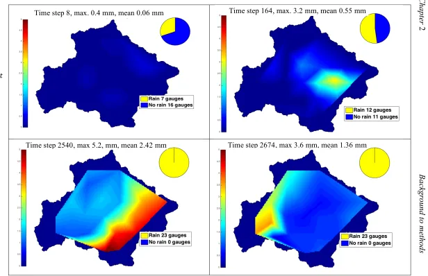
Figure 2-1: Maps of rainfall over the Brue catchment showing the variability in time and space. The brighter the color, the higher the rainfall. The pie chart at top right shows the proportion of gauges measuring rain in the illustrated time step (more yellow - more gauges with rain) ………..18

Figure 2-2 - Block diagram of a basic first order system ……….……….. 26

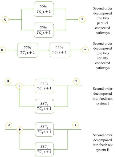
Figure 2-3 - Decomposition of a second order TF into first order systems connected by different pathways ………..……….. 27

Figure 2-4 - A schematic representation of a general identity system assuming a perfect model and a perfect inverse. In the ideal case, the system input U is identical to the system output Y* (adapted from Buchholz and Grünhagen, 2004) ………. 28

Figure 2-5 - The low-pass filtering (damping) effect of the catchment (storage) as the high frequency rainfall signal is converted into lower frequency discharge (adapted from Smith et al., 2004) …..……….. 39

Figure 2-6 - Definition of period and amplitude of a sinusoidal waveform ……... 40

Figure 2-7 - Phase shift and vertical shift of a sinusoidal function ………….………. 40

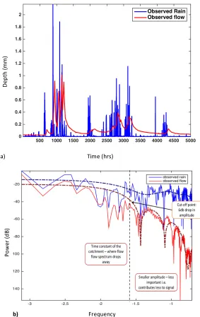
Figure 2-8: a) Time-series and b) frequency plots (periodogram) for the same set of rainfall and flow data. The periodogram pair shows the low-pass filtering effect of the catchment on the rainfall signal. The high frequency attenuation strength is illustrated in this double-logarithmic scaled graph ………..……….. 41

Figure 3-1 - Location and topography of the 8.8 km2 Blind Beck catchment, NW England ………..………... 46

(19)

xviii Figure 3-3 - a) The WISER water quality monitoring system at the main weir, Blind Beck Experimental Catchment, Cumbria, UK, b) The water-level recorder (left) and WISER water quality monitoring system (centre) at the main weir, Blind Beck Experimental Catchment, Cumbria, UK (Photos courtesy of: NA Chappell) ……….……… 47

Figure 3-4 - Saturated area close to the Low Hall stream gauging station within the Blind Beck Experimental Catchment, Cumbria, UK (Photo courtesy of NA Chappell) ………. 48

Figure 3-5 - Location of the 0.44 km2 tropical Baru catchment ………... 49

Figure 3-6 – 5-minute rainfall and flow data from the 0.44 km2 Baru catchment (February 1996) ………... 49

Figure 3-7: Images showing the character of the Baru catchment (Photos courtesy of N.A. Chappell and W. Tych) ……….…….. 50

Figure 3-8 - Brue catchment geology, location and gauge network. (Crown Copyright/database right 2016. A British Geological Survey/EDINA supplied service; National River Flow Archive, 2012) ………... 52

Figure 3-9 - The Brue catchment: The weir at Lovington (NRFA, 2012) and a typical river channel near Glastonbury. Upstream rain causes levels to rise and flooding when the embankments overtop. Flooded fields near Glastonbury (Edwin Graham, geograph.org.uk) ………..……….. 53

Figure 3-10 - Brue catchment showing how rain-gauges are grouped geographically for convenience. Colouring units are the Thiessen polygons ………...…. 55

Figure 3-11 - Cumulative rainfall for groups of rain-gauges (geographical grouping – see Figure 3-10) across the Brue catchment. Variation between gauges even over a 3-year period is obvious as is the similarity between FRAN, KNOW, MOWO and GODM, all situated at the southern edge of the catchment …... 56

(20)

Table of Figures

xix are characterised by frontal rainfall affecting the whole catchment, whereas summers tend to be characterised by much more localised storm events. Winters are wetter than summers (statistics shown in Table 3-4) showing that low intensity frontal rainfall actually produces more rainfall than the summer convective storms ………. 57

Figure 4-1: The use of Hammerstein-type non-linearity in the model identification (a) and inversion (b) processes where P is the observed rainfall, Pe is the effective rainfall, Q is the observed streamflow, Peh is the inferred effective rainfall and Ph is the inferred rainfall with the non-linearity reapplied ………...……. 60

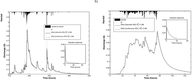
Figure 4-2: Measured and estimated streamflow for: a) Baru (at 5 minute intervals) and b) Blind Beck (at 15 minute intervals), together with the associated hyetograms and impulse responses ……….. 74

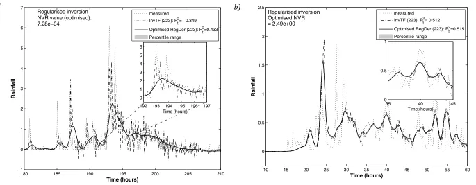
Figure 4-3: Comparison of rainfall simulated using the InvTF and RegDer (NVR optimised) methods for a) Baru and b) Blind Beck. Examination of the inset confirms that the RegDer method estimates the Baru catchment rainfall better (see Table 4-2) whilst there is little difference between the methods for Blind Beck rainfall. 99% uncertainty bands generated by Monte Carlo analysis are shown and can be seen to be very narrow ………. 75

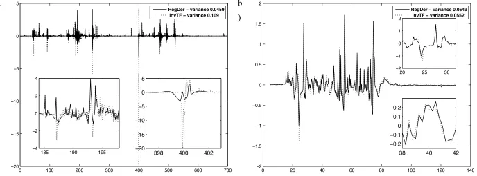
Figure 4-4: Comparison of residuals for a) Baru and b) Blind Beck for the two inversion methods showing the similarities in performance between the methods when used for Blind Beck (with a minor increase in noise for InvTF) and the differences when used for Baru (with large artefacts in InvTF) ……….…... 76

(21)

xx Figure 4-6: Comparison of the estimation of peaks for the two methods showing that for Blind Beck, both methods estimate the observed peak quite well with little difference between them whilst for Baru, the InvTF method hugely underestimates the peak whilst RegDer slightly over-estimates. The metrics PDIFF and PEP were taken from Bennett et al (2013) ………... 79

Figure 4-7: Outputs modelled from observed and modelled rainfall sequences for a) Baru and b) Blind Beck showing that the outputs (discharges) are indistinguishable over much of the figure despite the differing characteristics of the rainfall inputs ……… 82

Figure 5-1: a) The location of the 0.44km2 tropical Baru catchment in Sabah (dark grey area in bottom left map – Sabah Foundation Forest management concession), Borneo and b) the hydro- and hyetographs for the February 1996 sampled at 5 min intervals showing the flashy response of the catchment to the high intensity, spatially variable rainfall ………. 92

Figure 5-2: a) The location of the 8.8km2 temperate Blind Beck catchment in Northwest England and b) the hydro- and hyetographs for Blind Beck for the period from 26th Dec 2007 at 16:45 to 31st December 2007 at 21:45 sampled at 15 min intervals showing its response to less intense frontal rainfall and deeper hydrological pathways ………...…… 94

Figure 5-3: model identification and inversion workflow where P is the observed catchment rainfall, Pe is the effective rainfall, Q is the observed streamflow, Peh is the inferred effective rainfall and Ph the inferred catchment rainfall. Non-linearity is represented by the bilinear power law (Beven, 2012a, p91). The continuous time transfer function is given by G(s) where A(s) and B(s) are the denominator and numerator polynomials and the inversion process is represented by G-1(s) where A*(s) and B*(s) refer to the symbolic denominator and numerator polynomials of the regularised inverse transfer function as in (Equation 5-4) ……….. 96

(22)

Table of Figures

xxi Figure 5-5: Comparison of aggregated sequence to the Inferred effective rainfall sequence for a) Blind Beck (sampling interval 15 mins) b) Baru (sampling interval 5 mins) at aggregations of 4, 8 12 and 24 time periods (samples) illustrating how aggregation lowers the peak and spreads the volume of rainfall over a longer time period. The inferred effective rainfall sequence is plotted for comparison ……….……….. 104

Figure 5-6: The Rt2 and R tend to a maximum value as aggregation increases for a) Blind Beck and b) Baru. The resolution of the inferred effective rainfall is taken to be point at which the maximum is reached or very little change is apparent. For Blind Beck, this value is reached at 10 periods for both Rt2 and R. The result for Baru is not quite as clear but can be estimated to be 10 periods from R and 11 or 12 from Rt2 though Rt2 continues to increase up to 24 time periods perhaps due to higher variability of the rainfall ……....105

Figure 5-7: A similar plot to Figure 5-6 with aggregation by Moving Average for a) Blind Beck and b) Baru. Rather than reaching an asymptotic level, the Rt2_and R values maximize at 9 time periods for Blind Beck and 12 time periods for Baru (determined graphically in Matlab). These values have been used as the estimates of the resolution of the inferred effective rainfall and agree well with the estimates made by resampling. Convolution term in the caption is with reference to the method of calculating the moving average ………. 106

(23)

xxii Figure 5-9: Comparison of observed discharge and discharge generated from the Inferred Effective Rainfall for a) Blind Beck and b) Baru. The flow sequences match almost perfectly in the case of Blind Beck and very closely in the case of Baru where the peak flows are under-estimated. Note that the forward (rainfall-discharge) model fit for Blind Beck (98%) is better than for Baru (88%) (Kretzschmar et al, 2014) ……….……….. 110

Figure 6-1 – The variability in the rainfall field in space and time over the Brue catchment – brighter colours mean more rain (mm). Rainfall sampled at 15 minute intervals. The pie charts show how many gauges measure rain - the more yellow, the more gauges are measuring rainfall .………..112

Figure 6-2 - the model identification and inversion workflow showing the off-line non-linear transformation ……….114

Figure 6-3 - Brue catchment geology, location and gauge network. (Crown Copyright/database right 2016. A British Geological Survey/EDINA supplied service; National River Flow Archive, 2012) ……….… 116

Figure 6-4 - Comparison of modelled Rt2 (green bars) with inferred, aggregated Rt2 (red bars) for each individual gauge. (Crown Copyright/database right 2016. A British Geological Survey/EDINA supplied service; National River Flow Archive, 2012) ……….. 118

Figure 6-5 - Observed rainfall from example gauges comparing flow generated using the observed and inferred rainfall with the observed flow ………… 120

Figure 7-1 - Model identification and inversion workflow showing the off-line linear transformation ………..……… 127

Figure 7-2 - Brue catchment showing location of 23 gauges used in the study and the underlying geology. (Note that this map is also used elsewhere in a different context, so is provided here for clarity.) ……….. 130

(24)

Table of Figures

xxiii Figure 7-4 - 3 years of catchment average rainfall data sampled at 15 minute intervals for the Brue catchment plotted as water years - October 1994 to September 1997. Differences between years and between seasons are evident from these plots and from the statistics shown in Table 7-1 …… 132

Figure 7-5 - 3 years of flow data sampled at 15 minute intervals for the Brue catchment plotted as water years - October 1994 to September 1997. Differences between years and between seasons are evident from these plots and from the statistics shown in Table 7-1 ……… 133

Figure 7-6 - Key characteristics of the rainfall series showing the effect of increasing sampling period a) Standard deviation (mm), b) Lag-1 auto-correlation coeficient c) Skewness d) Kurtosis e) Proportion of wet time periods f) Maximum intensity (mm/hr)………...………...136

Figure 7-7 – Top plot – An example of rain at individual gauges (grey bars) over-plotted with catchment average rain (red bars); Bottom plot – the number of gauges with rain measured at each time period. The plots given an idea of the temporal and spatial variation in rainfall and illustrate how spreading rainfall evenly over the catchment lowers the rainfall peaks. This maybe the case even when all gauges have rain if some gauges have high rainfall and others low ……… 140

Figure 7-8 – Box plots of the 4 basic statistics, maximum rainfall intensity and proportion of wet time periods for the 23 gauges across the Brue catchment sampled at 15 minute intervals. The catchment average value is shown as a black + ………..……. 141

(25)

xxiv Figure 7-10 - A short section of hydrograph from WY3 showing missing peaks, extra peaks and badly reproduced recessions in more detail (blue: observed flow; red: predicted flow using CAR input) ……….…… 148

Figure 7-11: Cumulative rainfall for each water year. Variation in temporal patterns can be seen as changes in the shape of the CAR plot (red line). The grey lines show the cumulative rainfall measured at each gauge. The shape and range indicate how both spatial and temporal patterns vary from gauge to gauge and from year to year ………. 150

Figure 7-12a/b/c: Total rainfall over the Brue catchment in WY1 by gauge. The Thiessen polygons are coloured according to the rainfall at the gauge. Highest rainfall is on the higher ground to the north-east and lowest close to the catchment outlet……… 151/2/3

Figure 7-13a/b/c - Hydrographs simulated from rainfall measured at individual gauges (plotted in grey) over plotted by the observed hydrograph (blue line) for WY1. In many cases, the individual gauges over-estimate both the peak flow and the recessions. Also simulated peaks may be observed which do not occur in the observed hydrograph ……….……..…….……… 155/6/7

Figure 7-14a/b/c Spatio-temporal importance of the gauges is illustrated by plotting the fit of model unique to each rainfall-runoff combination on a catchment map. The theissen polygons are coloured according to the coding listed in Table 7-4. All gauges in WY1 are coded green – good fit (Rt2 > 0.80) with six over 0.9 so can be expected to be representative of the catchment as a whole. CAR model fit is 0.908 ………..………. 158/9/60

(26)

Table of Figures

xxv Figure 7-16a/b/c - Catchment average and inferred catchment average rainfall during the spring in each of the three years ……….………..167/8/9

Figure A2-1a WY1 – The longest time delays on permeable areas of catchment however the range is small, 24-26 15-minute time-periods ……… 175

Figure A2-1b WY1 – non-linearity generally decreases towards catchment outlet, ranging from 0.55 near the outlet to 0.65 as distance and elevation increase ………. 175

Figure A2-2a WY2 – Time –delay is shorter, further from the catchment outlet with 2 exceptions which lie on the permeable band. There appears to be no significant correlation with rainfall amounts (see Figure 7-12b) …...……. 176

Figure A2-2b WY2 – The pattern of non-linearity is the reverse of WY1 with lowest being furthest from the catchment outlet ………... 176

Figure A2-3a WY3 – Time delay generally decreases towards catchment outlet – with two exceptions. Rainfall generally follows the same pattern (see Figure 7-12c) ………...……….…. 177

Figure A2-3b WY3 – No distinct pattern is visible in the non-linearity. Rainfall generally decreases towards the outlet (see Figure 7-12c) occurring in much more defined bursts than in other years (see Figure 7-4) resulting in several distinct flow events unrelated to the seasons (see Figure 7-5)... 177

Figure B - 1: Cross-validation plots for WY2 and WY3 based on the model identified for WY1. The Rt2 fits are acceptable in both cases indicating the model for WY1 is a reasonable average model for the whole period. In WY3 the recessions are better reproduced than by the best-fit model for WY3 (Figure 7-9) ……… 179

Figure B - 2: Cross-validation plots for WY1 and WY3 based on the model identified for WY2. The Rt2 fits are acceptable in both cases indicating the model for WY2 is a reasonable average model for the whole period. In WY3 the recessions are better reproduced than by the best-fit model for WY3 (Figure 7-9) ……… 180

(27)

xxvi indicating the model for WY3 is a reasonable average model for the whole period over the whole performance range even though the recessions fit poorly in WY3. (Figure 7-9) ………...……….. 181

Figure C-1 – Comparison of model fits and hydrographs generated from ECAR (which could be an average of several gauges or an estimate from one gauge) and DGR for the same gauge or gauge-set. It can be seen that although for both the summer and autumn events the catchment average generates a good approximation of the observed hydrograph, it shows some peaks not present in the observed outflow hydrograph due to rain at gauges which are included in the ECAR but having no effect on the outflow. The Autumn event does not fit at all well and it can be assumed that several gauges are supplying misinformation, that is, adding significant amounts of rain to ECAR whilst not affecting the outflow.………..………. 184

Figure 8-1 - Model identification and inversion workflow showing the off-line linear transformation ………..………. 192

Figure 8-2 - Brue catchment showing location of 23 gauges used in the study and the underlying geology………..194

Figure 8-3 - Frequency plots of the DGR and the residual series CAR-DGR. DGR mirrors the flow and drops sharply at the frequency of the critical time constant of the catchment. All frequencies below the cut-off point – where the amplitude of the DGR has dropped by 6 dB – are low power and have no significant effect on discharge generation (shaded area) as these parts of the signal are filtered-off by the catchment dynamics ……….……… 196

Figure 8-4 – Comparison of CAR and DGR for a short section of record. DGR mirrors the flow but it is also obvious that the same amount of rain does not always generate the same amount of flow – non-linearity – due probably to the state of the catchment ………..……… 197

(28)

Table of Figures

xxvii frequency part of the rainfall spectrum with the same distribution as the modelled residual series. A digital filter is constructed based on the AR structure of the residual series. After some manipulation, the resulting rainfall sequence looks like rainfall, has a similar temporal and frequency structure to the observed rainfall ……… 198

Figure 8-6 – The rainfall construction model is based on the rainfall and flow series for WY1. Flow modelled using the best available estimate of CAR and the best-fit model is compared to the observed hydrograph. Rt2 of 0.904 suggests that the peaks and high flows are well matched but the Rt2L is lower suggesting that recessions are slightly less well captured. This is the benchmark with which to compare the performance of the constructed rainfall series for the same period. ……….……… 199

Figure 8-7 – Time domain plots of Discharge Generating Rainfall (DGR) (top plot), an estimate of the low frequency part of the signal. and the residual difference CAR-DGR (lower plot), an estimate of the high frequency part of the rainfall signal, for WY1 ……….………...200

Figure 8-8 – the auto-correlation structure of the residual series, IRES. The 95% confidence limits are shown in red. In this example, 13 correlation coefficients should be included to reproduce the correlation structure……… 201

Figure 8-9: Comparison of the distributions of calibration residuals (IRES) and simulated residuals (XIRES). Left hand plot – cumulative distribution function, right hand plot – frequency histogram (slightly enlarged to show detail around 0).……….………..……….. 202

Figure 8-10 – comparison of the series of simulated residuals (XIACF – blue line and blue bars) and base residuals (IRES – red line and yellow bars) shows them to have similar distributions ………..……… 202

Figure 8-11 – the top plot shows the series NR = ( _()'%&'

*∗ DGR) + XIACF

(29)

xxviii Figure 8-12 – Frequency spectra of NR (new rainfall sequence) and CAR are very similar in the area of interest showing that the auto-correlation structure has been maintained ……….………….… 205

Figure 8-13 - Frequency spectra of CAR and NRCV. The spectra show a slight vertical shift as a result of the rescaling of the rainfall series but the frequency patterns remain unchanged ……….…… 205

Figure 8-14 – Hydrograph generated from constructed rainfall series NRCV compared with the observed hydrograph. An Rt2 of 0.930 is better than the hydrograph generated from observed rainfall. The Rt2L value confirms that fit is good over the whole flow range ……….………...……… 206

Figure 8-15: Discharge generated from pure DGR plotted against discharge generated from a constructed rainfall series (correlation coefficient = 0.968) showing that the constructed series does generate the correct hydrograph. ………... 207

Figure 8-16 – comparison of hydrographs generated from the DGR inferred from the CAR and DGR inferred from NRCV. The fits are almost identical confirming that although the rainfall pattern is different, the discharge generating characteristics have been preserved ……… 209

Figure 8-17 - 50 possible rainfall realisations (grey bars) compared with the observed rainfall series (red dotted bars) and the observed flow (blue line, bottom plot) and hydrograph generated from the mean of 50 realisations (light blue line in bottom plot). Rt2 between observed flow and simulated hydrograph is 0.963. Enlarged section of the plot are shown in Figure 8.18 ………..………..………. 211

(30)

Table of Figures

xxix and 0.810 for the recession plot indicating that the process works best where there is active flow……….………… 212

Figure 8-19: Hydrographs simulated from 50 rainfall realisations (grey lines). The hydrograph simulated from the mean of the 50 rainfall realisations is plotted in black and the observed hydrograph in blue …..………... 213

Figure 8-20: Rt2 values for the hydrographs plotted from each rainfall realisation (blue circles). Also shown, for comparison, are the Rt2values for hydrographs simulated from the observed rainfall and the average of the rainfall realisations ………… 214

Figure 8-21 – Observed rainfall and flow time-series with a gap in the rainfall (WY1-WY3). The observed rainfall over the gap is shown for comparison with the generated rainfall ………..……….………… 215

Figure 8-22: Hydrographs modelled from observed rainfall in the calibration period (top plot) and from reconstructed the rainfall model (bottom plot) ………. 216

Figure 8-23 – Gap in WY2 (length 10000 time periods) in-filled by DGR generated from flow and model fitted to calibration time-series. The calibration series is effectively WY1 ………...……….……… 217

Figure 8-24 - Top plot shows the observed rainfall with the in-fill over plotted. The bottom plot shows just the in-filled series ……….………... 218

Figure 8-25 - Hyetograph of in-filled rain and the hydrograph generated from it over the gap (top plots) and the hyetograph and hydrograph for the full record with the gap filled ………... 219

(31)

(32)

List of Tables

xxxi

List of Tables

Table 3-1 – 15-minute rainfall and flow statistics for 26th - 31st December 2007 in the Blind Beck catchment……….47 Table 3-2 - Statistics of 5-minute rainfall and flow for February 1996 ... 50 Table 3-3 - Statistics for the Brue catchment October 1994 - September 1997. Rainfall statistics for each rain-gauge. Gauges are grouped geographically (see Figure 3-10) ... 54

(33)

(34)

List of Tables

xxxiii storms can be seen to have very different characteristics a) is a short-lived summer convective cell that passes mostly over the eastern side of the catchment. Storm b) is a more widespread over the catchment with the heaviest rain to the northeast. Storm c) is a widespread event with a heavier core falling mostly on the northern side of the catchment but with a few southern gauges measuring more rain ………...….... 183 Table C-2 – Model fits for a selection of gauges for each of the example events. The hydrograph generated from ECAR for the summer event shows a good fit to the Qobs as do each of the sample gauges. The Qinv hydrograph shows an improved fit. The Qsim hydrograph for the winter event shows a slightly less good fit and one of the individual sample gauges shows less good fit. The autumn event shows a poor fit to ECAR. Two of the sample gauges show a poor fit that is only partly resolved by using the DGR ……… 185 Table 8-1 – Proportion of zero rainfall periods in CAR is 0.809. Adjusting the threshold

(35)

1

Chapter 1 Introduction

1.1. Flooding and climate change

Floods are the most common and often the most destructive of natural disasters. Almost everywhere on Earth where it rains is vulnerable to flooding. Although flooding is most commonly a result of heavy rainfall, it can be caused by rivers, dam failures, changes in groundwater, inadequate drainage (sewer flooding), rapid ice-melt or coastal flooding in the form of extreme high tides and or storm surges and combinations of these (Dale, 2005). Most floods take time to evolve giving time for areas likely to be affected to be evacuated, however fast developing and flash floods are highly damaging, destructive and dangerous and leave little time for defensive measures to be taken. The consequences of flooding are aggravated by man’s wish to live close to water and the building of both commercial and residential property on natural floodplains (Merz et al., 2010). Due to climate change, extreme flood events are expected to occur more frequently (Huntington, 2006) and a warmer climate means that the atmosphere can carry more moisture with more energy available to generate more extreme storms. Heavy rainfall, snowfall and heatwaves have become more frequent (Royal Society, 2017) and the frequency of floods has increased (Milly et al, 2002). Attributing individual events to anthropogenic warming is difficult due to natural variability, however exposure to flooding is likely to increase as the degree of warming increases (Hirabayashi et al., 2013) and short-term regional variations become more extreme. It is becoming apparent that atmospheric rivers play an important role in storms and floods in the Pacific south-west US (Dettinger, 2011) whilst many of the largest winter flood events in the UK have been linked to atmospheric rivers (Lavers et al., 2011) including Storm Desmond which brought record rainfall and river levels and severe disruption to the northern UK in December 2015 (JBAtrust, 2016). The projected increases in extreme rainfall and associated flooding mean that accurate predictions of rainfall and streamflow will become even more important in the future. It is unlikely that flooding can be eliminated, the challenge is to manage and reduce the risk (Shaw et al., 2011).

(36)

Chapter 1 Introduction

2 time and space. The total amount of rainfall over a catchment is important but so is its spatial location and intensity as it may affect localised flood risk and operational decisions such as flow releases from reservoirs (Croke, 2006) or estimation of over-bank flows. Linsley (1967) stated that, if the right data is available, streamflow hydrographs can be generated that are as accurate as the input data. Rainfall is the major input and has the greatest variability so how well the hydrograph can be simulated may be dependent on how well the variation is understood and can be defined (Xu and Singh, 1998).

Deriving the relationship between rainfall and flow is a fundamental problem (Xu and Singh, 1998) not least because many of the processes of water flow in a catchment take place underground and are difficult or impossible to measure (Beven, 2012a). Much of what is understood about these processes is inferred from point measurements which, due to variability, only provide a limited picture of what is happening (Cole and Moore, 2008). How a catchment responds varies from event to event or even within the same event due to variations in antecedent conditions and the type of storm (Chappell et al., 2017b). The heterogeneity of catchment characteristics interacts with rainfall properties such as intensity, volume and storm movement resulting in different areas of the catchment generating different amounts of flow (Shankar et al., 2002). Catchment characteristics may include antecedent wetness, topography, soil types and structures, regolith and rock types, channel density and human influence. Not all rainfall contributes directly to the storm hydrograph as some is lost by evaporation.

1.2. Flow generation processes and pathways

(37)

3 is the result of overland flow. Overland flow does not occur everywhere but is the main mechanism in impervious areas. Saturation excess runoff (Dunne and Black, 1970) is a rapid transport mechanism where soils are saturated by emerging sub-surface outflow or perched water tables. It may occur with subsurface flow, the relative importance of each being dependent on the catchment and precipitation rates. Lowdermilk (1934) and Hursh (1936) suggested that sub-surface flow could be the main storm flow generation mechanism. Later studies suggested it might be the only mechanism (Hewlett and Hibbert, 1963; Whipkey, 1965). Weyman (1970) showed that soil did not have to be completely saturated for saturation excess contributions to occur but could be a result of lower soil horizons having a reduced permeability. Sub-surface pathways include preferential flow paths through percolines (a network of old root channels, soil cracks and animal burrows - Bunting, 1961) and soil pipes (Beven and Germann, 1982) that by-pass slower mechanisms such as flow through the soil matrix. Sub-surface flow may also occur along boundaries between permeable and less permeable layers (Bonnell and Gilmour, 1978). None of these mechanisms are mutually exclusive and they may occur in different parts of the catchment at different times or in different areas during the same storm (Dunne, 1978). The original assumption was that storm runoff was due to water generated by the current event. Work using tracers (Sklash et al., 1996) revealed that some flow comes from displaced ‘old’ water that has previously been stored and is rapidly released during a storm event (Kirchner, 2003). This concept has importance for the understanding of hillslope hydrology, water quality variations and the ecological impact of storms.

(38)

4 within the catchment, that is, the time taken for runoff to reach the measurement point (McDonnell, 2003).

1.3. Scaling and measurement in space and time

The timescale of a rainfall-runoff relationship should be determined by its purpose, for instance, a monthly or annual time-step may be adequate for determining overall catchment water yield. However measurements may need to be made at a much smaller interval then aggregated in order to get accurate estimates at the required time period. This may be particularly important in small catchments or those susceptible to flash flooding. If flood peak or water quality assessment is the purpose, then small time steps are also required so that the detail can be captured (Chappell et al, 2017a). The effects of sparse data sampling (in both space and time) are a major source of uncertainty in rainfall-runoff relationships (Kavetski et al, 2011). Catchment size also has an effect with both small relatively homogeneous catchments (for example, urban areas) and large catchments over long time periods, where local variations in rainfall and runoff are smoothed out, having relatively simple rainfall-runoff relationships. More generally, intermediate size catchments measured at short time periods with intermittent rainfall and variations in catchment characteristics show complex, non-linear relationships (Shaw et al., 2011).

(39)

5 assumptions (Jakeman et al, 1990). Whatever model is used; its predictions are only as good as the input data (Shaw et al., 2011).

Thus, it can be seen that it is important to have reliable estimates of the rainfall over a catchment. It is often the case that a single rain-gauge or a sparse rain-gauge network is assumed to represent the spatially and temporally variable rainfall field. The design and density of rain-gauge networks has been the subject of research over a long period and was one of the drivers for the set-up of the Brue experimental catchment (Bell and Moore, 2000). Rain-gauges may also be subject to measurement errors, for example, under-catch (Pollock et al, 2014) and can only provide a measurement of rainfall over a limited area that may or may not be representative of the rainfall over the whole catchment. The rain that falls on the catchment that becomes streamflow can be measured at the outlet. The measured streamflow contains information not just about the rainfall but the way the catchment damps the rainfall signal as it is converted to streamflow. If this information could be extracted, it might be possible to improve rainfall forecasts and thus provide less uncertain flood predictions. Existing methods for estimating catchment rainfall, for example, the Thiessen polygon approach (Shaw et al., 2011, p167) only make use of the rainfall signal. Thiessen weights for each rain gauge are computed by their relative area of influence and the area of each polygon used to weight the rainfall amount of the station in the center of the polygon. If any station is missing, the polygons must be recalculated. Thiessen polygons do not take elevation effects into account and are not related to streamflow generating processes (Schumann, 1998). Reverse hydrology takes the information present in the streamflow, that incorporates catchment information, and uses it to infer the rainfall that generates the discharge and thus could result in a better estimate of the flow hydrograph.

1.4. Hydrological modelling – a brief introduction

(40)

6 ungauged catchments or into the future to assess the effects of change, as compensation for weaknesses in measurement techniques. It is often very difficult or impossible to measure all the processes and states required to describe and understand the system, for example, storage. Modelling for research purposes aims to improve understanding of the processes involved in the hydrological system with most being learnt when the data does not support existing theories which then have to be modified (Beven, 2012a). The ultimate aim of most modelling is to improve decision making in, for example, water resource management, flood control, pollution mitigation or to supply boundary conditions to atmospheric circulation models (Wagener et al, 2004).

Models range from physics-based distributed models, with many parameters that try to reproduce the heterogeneity of the catchment characteristics and hydrological processes, to black-box models with very few parameters based only on the observations of inputs and outputs without any reference to physical reality of the processes involved. In between these extremes are lumped physics-based models that assume that the processes and characteristics can be averaged over the catchment, and grey-box models based on the relationship between the system inputs and outputs but with some physical interpretation. Data-based mechanistic (DBM) modelling used in this study falls into the latter category (see section 2.4).

(41)

7 investigate the effects of land-use change on flooding or water quality (Abbott et al., 1986).

Semi-distributed models lump the characteristics of similar areas of catchments together (may be described as Hydrological Response Units (HRUs) - Flügel, 1995). This has the effect of reducing the number of parameters that need to be estimated. HRUs may be defined using GIS data. A grid-based approach can also be used where calculations are made based on every grid element, for example, LISFLOOD (De Roo et al, 2000). Parameters are averaged for each HRU or grid so they can be thought of as a collection of small scale lumped models (Beven, 1989). HRUs can be mapped back into space using GIS but scale dependence of the parameters and calibration can be a problem (Vinogradov et al., 2010).

Lumped physics based models regard the catchment as a single unit using average parameter values that are assumed to be representative of the whole catchment. They have only a few parameters however spatial variation cannot be represented by a single value (Sharma and Luxmoore, 1979). Calibration can be automated but there is a danger of over-parametrisation and problems may be caused by parameter inter-action (Ibbitt and O’Donnell, 1971). It has been suggested that 5 parameters explain most of the information contained in hydrological data (Hornberger et al., 1985).

(42)

8 Not only the time-step but also the choice of model should be defined by the purpose of the modelling exercise. If the aim is to predict discharge from rainfall without any consideration of the processes involved, then a simple black box model may be good enough. Black box models are usually lumped at catchment scale and, in contrast to distributed physics based models only have a very few parameters. These models attempt to extract as much information as possible from the available data by relating the inputs to the outputs, that is, the problem becomes one of systems analysis (Young, 1998). It can be argued that the data may not be good enough to identify a complex highly parameterised model (Jakeman and Hornberger, 1993) so successfully transforming the inputs into outputs without any knowledge of the processes by which this occurs is good enough. This is data-based modelling. It is dependent on suitable data being available so this approach could not be used in ungauged catchments. The concept has been extended by suggesting that the models identified should have some physical explanation (Young and Beven, 1994). The objective approaches used in black box modelling are used to identify a range of parsimonious models from the data. Only models that have a physical interpretation are retained (Young and Lees, 1993). This is Data-Based Mechanistic modelling. It combines elements of white box, physics based models with black box techniques and is often termed grey box modelling (Lees, 2000).

As models are approximations of the real world (Oreskes and Belitz, 2001) they have built-in uncertainties which may include the modeller’s perception of the system, the simplifications involved in building the mathematical model, model structure, parameter estimates, the scale of the processes involved (do micro-level physical laws apply at catchment scale?), the time interval (does a model that has been calibrated for one time interval apply to another?), spatial scale (does a model calibrated for one catchment apply to another one?), the non-linearity of hydrological processes and the quality of the data. In order for the results from the modelling process to be useful, some measure of the uncertainties involved is needed to supply some indication of the limitations to its applicability. These uncertainties must be communicated in a way that is easily understandable to the non-expert.

(43)

9 Figure 1-1. The perceptual model is the ‘Big Picture’ in the mind of the modeller. It will be unique to the individual, being the way they perceive the complexity of the hydrological system. The conceptual model is the mathematical simplification of this concept and the procedural model is the code needed to run it. Calibration uses observed data to determine model parameters whilst evaluation may use a different set of data to evaluate whether the model produces acceptable results. Measures used to assess model performance may be objective, for example, the Young Information Criterion (YIC) (Young, 1984, 2011) or Nash-Sutcliffe Efficiency (Rt2_{or NSE) or subjective based on} the experience of the modeller with reference to the model’s purpose. Acceptance requires not just that a model is a good fit but also has a physical explanation. If the criteria for acceptance are not met at any stage, then modifications may be made and the model reassessed. It can be argued that it is not possible to prove that a model is valid, only that it is wrong - the concept of falsification (Wagener et al, 2004).

Figure 1-1: Schematic showing the steps in model development/ selection in order of increasing approximation (adapted from Beven, 2012a)

DBM modelling takes a top-down approach to model identification and parameter estimation. Models are identified from the data (in this study, rainfall and streamflow) that have as few parameters as are necessary to adequately define the dominant processes of the (hydrologic) system. Model structure is identified using objective systems analysis methods that minimise the bias introduced by prior assumptions (Taylor et al., 2007) and enable the dominant modes of a system to be identified (Ockenden, 2010). Models are only accepted if they have a physical explanation (Young and Beven, 1994). DBM modelling often makes use of linear transfer functions however no real-world process is truly linear although it may be treated as such over a limited range of conditions (Leedal, 2006). If this is not the case, some means of

The Perceptual

Model

The Conceptual

Model

The Procedural

Model

Calibration EvaluationModel

Model Acceptable

?

Increasing approximation

N

(44)

10 accounting for the non-linearity must be applied before identifying the parameters of the linearised system.

1.5. Why reverse hydrology?

Managing and reducing flood risk is becoming more important due to man’s increased vulnerability. Deriving a relationship between rainfall and flow is key but extremely complex and, because many of the processes involved are unmeasurable, often inferred from point or laboratory measurements. It is necessary to think laterally about the way models are identified and novel approaches such as the one presented in this thesis are necessary to provide new insights into the processes and their identification. Although rainfall is the key driver and often the major input to hydrological models, it is only part of the story. Streamflow contains information about both the rainfall and the catchment processes that generated it. Inversion utilises the information in both rainfall and streamflow so could be a tool to aid improved understanding of flow generation and its links to rainfall, leading to more reliable flood predictions.

(45)

11 takes streamflow as its input and generates rainfall as its output) because it is numerically poorly defined, particularly for non-linear systems, and, very importantly, because the catchment processes involve differentiation in both space and time. A forward model, linking the conversion of rainfall to streamflow, must first be identified and inverted to obtain a reverse model. Reverse hydrology does ‘hydrology backwards’ using an inverted model allowing rainfall to be inferred from streamflow (Kirchner, 2009).

Reverse hydrology takes the information present in the streamflow that incorporates catchment information, and uses it to infer Discharge Generating Rainfall for the catchment. Accurate streamflow hydrograph simulation depends on the availability of highly sampled rainfall data and also its spatial distribution (Littlewood and Croke, 2013). Estimating the short-term rainfall characteristics which are important in producing the hydrograph (Obled et al., 1994) may be useful for filling gaps in existing rainfall records, for example, due to equipment malfunction or periods when snow is the dominant precipitation (Hudson et al, 1997), where corresponding flow records exist and extending rainfall series for catchments which have long streamflow but only short rainfall records.

(46)

12 preference to ‘effective’ rainfall here because the bi-linear transform has been applied to the rainfall data so that a linear TF can be identified. Effective rainfall is defined by Beven (2012a) as the part of the rainfall that is equal to the volume of streamflow generated. This is not the same as the linearised rainfall calculated here.

Continuous time models are used because their parameters have a direct physical interpretation and allow a wide range of system dynamics typical of hydrological systems to be modelled – so called ‘stiff’ systems where there is a wide range in the time constants (Young, 2010). Given that sampling is frequent enough to capture the system dynamics, parameters are not sampling interval dependent. The rational transfer function model is trivially inverted (c.f. section 2.5 and Chapter 4). Where the resultant model would be ‘improper’, that is, the order of the numerator of the CT-TF is greater than that of the denominator, the inversion requires derivatives of the streamflow. Regularised Derivatives are used, hence the algorithm has been called RegDer. Application of the regularisation procedure (described in sections 4.2 and 4.3) makes inversion possible without amplification of the noise in the inferred rainfall series. The general approach used could be applied within any DBM or top-down modelling framework.

(47)

13 Possible applications and benefits of reverse hydrology include:

1) Filling gaps in rainfall records

2) Assessing rain-gauge networks (no. and position of gauges) 3) Identifying inconsistent or uninformative rainfall or flow data 4) Improved understanding of catchment processes

5) Improved understanding of rainfall distribution

6) Extraction of the essential rainfall dynamics required to generate flow from the broad-spectrum input signal.

(48)

14

1.6. Aims and objectives

This study aimed to:

1) Improve understanding of the information content of space-time distributed rainfall data for flood modelling

2) Develop tools and techniques for improving rainfall datasets for catchment modelling

These aims will be met by the following objectives:

1.i Develop a new method for inferring rainfall from sub-hourly streamflow data based on a novel regularisation technique

1.ii Evaluate the regularisation technique by comparison with existing inversion methods utilising data from two catchments with contrasting rainfall characteristics and flow-paths using a range of metrics

1.iii Assess the ability of the regularisation technique to capture the dominant modes of the rainfall-runoff behaviour using methods of temporal aggregation and spectral analysis

1.iv Assess the ability of the regularisation technique to capture the spatio-temporal structure of catchment rainfall

2.i Quantify local rainfall records that are misinformative for flood modelling 2.ii Quantify the spectral components of the rainfall signal responsible for flood

generation

2.iii Develop a new technique for in-filling and extending rainfall records based on a combination of regularisation and spectral decomposition

1.7. The story so far ...

This thesis is based on a number of articles, either already published or prepared for publication (Chapters 4-8):

(49)

15 Chapter 4 (Kretzschmar et al., 2014) presents the novel inversion method utilising regularised derivatives (RegDer) and compares it with an existing method using the direct inversion of a discrete transfer function (InvTF). Tests are carried out using data from two contrasting catchments – the tropical Baru catchment in Borneo and the temperate Blind Beck, a tributary of the River Eden, in North-west England. Using both methods, the hydrograph generated from the inferred rainfall is much closer to the observed hydrograph than one generated using the forward model. However, the direct inverse method shows evidence of high frequency artefacts which would cause it to fail the criteria for DBM modelling. The output from the RegDer method shows evidence of loss of resolution however tests show that the essential catchment dynamics are being captured.

This theme is continued into Chapter 5 (Kretzschmar et al, 2015) where spectral analysis was used to confirm that despite the loss of time resolution in the rainfall output from the RegDer method, the catchment dynamics necessary for streamflow generation are being captured. Estimates of time resolution from spectral analysis are compared with estimation of the time resolution from aggregation of the observed rainfall time-series. Both confirm that the essential dynamics are being captured and that the loss of resolution is the price paid for numerical stability of the inversion process.

Chapter 6 (Kretzschmar et al., 2016) continues this topic but this time applied to the heavily instrumented Brue experimental catchment in south-west England. The spatial element of catchment rainfall is picked up and it is demonstrated that the loss of time-resolution and representation of the essential rainfall characteristics applies everywhere in the catchment.

(50)

16 indicate its representativeness. A hydrograph generated using DGR shows an improved fit to the observed hydrograph over using a forward model and observed rainfall.