On the integration of due date setting and order release control

1

On the Integration of Due Date Setting and Order Release Control

Matthias Thürer (corresponding author), Martin J. Land, Mark Stevenson and Lawrence D. Fredendall

Name: Dr. Matthias Thürer

Institution: Jinan University

Address: Jinan University No 601, Huangpu Road 510632 Guangzhou – PR China Email: [email protected]

Phone: +86 15916317887

Name: Dr. Martin J. Land

Institution: University of Groningen Address: Department of Operations

Faculty of Economics and Business University of Groningen

9700 AV Groningen – The Netherlands

Email: [email protected]

Phone: +31 503637188

Name: Dr. Mark Stevenson

Institution: Lancaster University

Address: Department of Management Science Lancaster University Management School Lancaster University

LA1 4YX – U.K.

Email: [email protected]

Phone: +44 1524593847

Name: Professor Lawrence D. Fredendall

Institution: Clemson University

Address: Department of Management

101 Sirrine Hall

Clemson SC – United States

Email: [email protected]

+1 8646562016

2

On the Integration of Due Date Setting and Order Release Control

Abstract

This paper calls for a paradigm shift in the production control literature away from assuming due date setting and order release are two independent decision levels. When order release is controlled, jobs do not enter the shop floor directly but are retained in a pre-shop pool and released to meet certain performance targets. This makes the setting of accurate planned release dates – the point at which jobs transition from the pool to the shop floor – a key consideration when setting due dates. We develop a new approach to estimating planned release dates to be embedded in the Workload Control concept. Our approach is unique as it anticipates the release decision as part of the due date setting procedure. This makes a second independent release decision superfluous and avoids a major cause of tardiness – deviations between (i) the planned release date used when calculating the delivery time allowance and (ii) the actual, realized release date. Simulation is used to compare the performance of Workload Control using two decision levels with the new single-level approach where the release decision is anticipated when setting the due date. Performance improvements are shown to be robust to uncertainty in processing time estimates.

3 1. Introduction

This study examines the performance of due date setting and order release control in job shops. A basic assumption within the production planning and control literature is that due date and order release decisions are taken sequentially and independently. In other words, it is assumed that due dates are set first and then jobs flow into a pre-shop pool to await the release decision. This study questions this fundamental assumption. We argue that, rather than taking these two decisions independently, the release decision should be an integral part of the due date setting procedure.

Most literature on the estimation of due dates or delivery time allowances in job shops assumes the immediate release of jobs, i.e. that the delivery time is given by the time a job spends on the shop floor only (e.g. Weeks, 1979; Ragatz & Mabert, 1984; Ahmed & Fisher, 1992; Vig & Dooley, 1993; Moses et al. 2004; Thürer et al., 2013). This has limited applicability to shops where the release of jobs is controlled. When order release is controlled, jobs do not enter the shop floor directly. Instead, they are retained in a pre-shop pool and released using criteria that allow the shop to achieve certain performance targets, e.g. to restrict the level of work-in-process inventory and/or maximize due date adherence. Consequently, the realized delivery time is split into two parts: (i) the time a job waits in the pre-shop pool prior to being released (i.e. the pool waiting time); and, (ii) the time a job spends on the shop floor (i.e. the shop floor throughput time). Both elements contribute to the overall delivery time and should therefore be considered when setting delivery time allowances or due dates to ensure that they are both competitive and feasible (Thürer et al., 2014a). This makes the setting of accurate planned release dates – the point at which jobs are transferred from the pre-shop pool to the shop floor – a key priority (Thürer et al., 2016).

Workload Control – a production planning and control concept specifically developed for job shops (Kingsman et al., 1989; Zäpfel & Missbauer, 1993; Kingsman & Hendry, 2002; Stevenson

4

setting procedure. Since a release decision is already taken when due dates are set, it is argued that another, independent release decision becomes superfluous. Jobs can simply be released on their planned release date, which can be determined as part of the due date setting procedure. This integrates the release decision into the due date setting procedure and avoids variability between the planned release dates used to determine delivery time allowances and the release date actually realized.

This paper has the following two objectives:

1. To develop a new approach to calculating planned release dates that anticipates future release decisions, which can be integrated into Workload Control’s due date setting procedure.

2. To assess the performance of Workload Control based on two independent decision levels – one for delivery time estimation and one for order releases – and based on one decision level, where jobs are released on their planned release dates, which makes the release decision an integral part of the due date setting procedure.

The remainder of this paper is structured as follows. Section 2 reviews the literature to identify the Workload Control due date setting procedure and order release method to be considered in our study. Section 3 then develops a new approach to effectively estimating planned release dates. A simulation model to assess performance is presented in Section 4 before simulation results are presented in Section 5. Finally, the paper concludes in Section 6, where future research directions are also outlined.

2. Literature Review

Section 2.1 provides a brief overview of how due dates are set in the literature on job shops in general and outlines Workload Control’s due date setting procedure – the procedure into which our new approach to setting planned release dates will be integrated. Workload Control’s load-limiting order release method is then outlined in Section 2.2. This method determines the structure of our new approach to setting planned release dates since it is the release dates realized by this method that we have to predict.

2.1 Due Date Setting Rule

5

the due date is specified by the customer and, therefore, reasonably fixed (e.g. Ragatz & Mabert 1984; Cheng & Gupta 1989; Kingsman 2000). The main focus of this study is on setting due dates and thus on the former. A feasible due date (d_j) is generally determined by forward scheduling when a new job j arrives by summing the following three elements to the current time

t (see Equation (1)): an allowance _j for the time that a job has to wait in the pre-shop pool prior to release; an allowance _ij for the operation throughput time of each operation i in the routing

j

R of a job to allow for the shop floor throughput time; and, an external allowance _j that compensates for variability between the estimated lead time and the delivery time that is ultimately realized. The process of setting each of these three allowances is outlined in the following three subsections.

j R

i ij j

j

j

t

d   





(1)

2.1.1 Setting Allowances for the Pool Waiting Time

The literature on due date setting rules typically assumes that jobs are released immediately, i.e. that the pool waiting time _j is zero. Similarly, the Workload Control literature that has considered the estimation of due dates and order release simultaneously assumes that the pool waiting time is either zero (e.g. Enns, 1995a; Ahmed & Fisher, 1992) or constant for all jobs (Hendry et al., 1998; Thürer et al., 2013 and 2014a). To the best of our knowledge, the only study to date to present a method that estimates a dynamic allowance for the pool waiting time was presented by Land (2009). Following Little’s Law (Little, 1961), Land (2009) estimated the pool waiting time based on the total processing time units waiting in the pool to be released to the station that is most likely to restrict the release of a job, i.e. the station that had the largest load waiting to be released across the stations in the routing of a job. The pool waiting time is given as the quotient of this maximum pool load and the maximum output of the station. Land’s (2009) approach will be included as a benchmark for the new approach to calculating pool waiting times – and thus planned release dates – developed in this study.

2.1.2 Setting Allowances for Operation Throughput Times

6

determined for operation throughput times. For example, forward infinite loading assumes operation throughput times are constant (e.g. Weeks, 1979; Ragatz & Mabert, 1984; Vig & Dooley, 1993). Meanwhile, other studies link the processing time and shop load to the delivery time based on historical data via regression (e.g. Ragatz & Mabert, 1984, Ahmed & Fisher, 1992; Vig & Dooley, 1993; Moses et al., 2004) or link the workload at a station to the allowance for the operation throughput time (e.g. Nyhuis & Wiendahl, 2009).

Bertrand (1983a and 1983b) determined a dynamic allowance for operation throughput times by successively scheduling operation due dates dij for each operation i in the routing of a job j,

where d0_j is defined as the current date. Using the time-phased accepted workload (

A st

W ) and time-phased capacity ( C_st ) of the corresponding station s – both measures calculated cumulatively up to time bucket t – the operation due dates are calculated as follows. Starting

with the first station in the routing of a job:

 If the time bucket into which the operation due date would fall if capacity were infinite – that is dij di1j  pij – has enough free capacity to include the workload pij of the i

th

operation of job j at the relevant station s – that is W_stA p_ij C_stu_swith us equal to the utilization rate –

then the operation is loaded into the time bucket and the operation due date is given by this time bucket.

 If no or insufficient capacity is available, the next time bucket t+1 is considered until the workload has been successfully loaded.

This procedure is then repeated at the next station in a job’s routing until all operation due dates have been determined. An operation remains loaded into a time bucket – and thus contributes to the cumulative workload – until it has been completed.

This forward finite loading procedure was recently identified as the best solution for the Workload Control concept (see, e.g. Thürer et al., 2013) and will thus be included in our study to set allowances for operation throughput times.

2.1.3 Setting an External Allowance to Compensate for Variability

7

production) due date and an external (or customer) due date – which is the internal due date plus the external allowance – are the studies by Bertrand (1983a), Enns (1995b) and Hopp & Sturgis (2000). The latter compared the use of a constant external allowance with the use of alternative, dynamic external allowances. Numerical results suggested that there are no significant performance differences between the use of a constant allowance and the best-performing dynamic allowance approach. In general, the external allowance accounts for any unforeseen variability. If it were predictable – as assumed when a dynamic external allowance is calculated – it would be better to incorporate this into the allowances for the pool waiting time and/or operation throughput times. This makes the use of a constant external allowance an effective option in practice. Workload Control uses an explicit constant external allowance since its forward finite loading procedure estimates an internal due date.

2.2 Order Release Control

There are many order release methods in the Workload Control literature; for examples, see the reviews by Wisner (1995), Land & Gaalman (1996), Bergamaschi et al. (1997) and Fredendall et al. (2010). In this paper, the LUMS COR (Lancaster University Management School Corrected Order Release) method is used as the basis for further developments because it was recently shown to be the best order release solution for Workload Control in practice (Thürer et al., 2012). LUMS COR uses a periodic release procedure executed at fixed intervals to control and balance the shop floor workload. This procedure keeps the workload R

s

W released to a station s

within a pre-established workload norm, as follows:

(1) All jobs in the set of jobs J in the pre-shop pool are sorted according to their planned release date, as calculated at customer enquiry management.

(2) The job jJ with the earliest planned release date is considered for release first.

(3) Take Rj to be the ordered set of operations in the routing of job j. If job j’s processing time

pij at the ith operation in its routing – corrected for station position i – together with the workload WsRreleased to station s (corresponding to operation i) and yet to be completed fits

within the workload norm C s

N at this station, that is ij W_sR N_sC i

p



8

is selected for release. That means it is removed from J, and its load contribution is included, i.e.

i p W

W_sR : _sR  ij iR_j.

Otherwise, the job remains in the pool and its processing time does not contribute to the station load.

(4) If the set of jobs J in the pool contains any jobs that have not yet been considered for release, then return to Step 2 and consider the job with the next highest priority. Otherwise, the release procedure is complete and the selected jobs are released to the shop floor.

A released job contributes to R s

W until its operation at this station is completed. Early studies on Workload Control typically focused on comparing the aggregate load of a station, i.e. the sum of all of the processing times of jobs released but not yet completed at a station, against an upper workload limit or norm (e.g. Bertrand & Wortmann, 1981; Hendry & Kingsman, 1991). But this ignored variance in the amount of upstream work (i.e. the indirect load), which is dependent on the position of a station in the routing of jobs. Therefore, the load contribution to a station in LUMS COR is calculated by dividing the processing time of the operation at a station by the station’s position in the job’s routing. This “corrected” aggregate load method (Oosterman et al., 2000) recognizes that a job’s contribution to a station’s direct load is limited to only the proportion of the total time the job spends on the shop floor that it is actually at the station.

In addition to the above periodic release mechanism, LUMS COR incorporates a continuous

workload trigger. If the load of any station falls to zero, the first job in the pool sequence with that station as the first in its routing is released irrespective of whether this would exceed the workload norms of any station. The continuous trigger avoids premature station idleness (see, e.g. Kanet, 1988; Land & Gaalman, 1998). When the continuous workload trigger releases a job, its workload contribution to a station is calculated using the same corrected aggregate load approach as used for the periodic release time element of LUMS COR.

3. Integrating Due Date Setting and Order Release Control

9

3.1 A New Procedure for Calculating Planned Release Dates

From the formalization of our release procedure in Section 2.2, it can be observed that three variables determine the final release date of a job: the corrected workload contribution of the job, the released workload, and the workload norm. The estimation of processing times – and thus the corrected workload contribution – cannot be influenced by production control. Meanwhile, the workload norm is a variable that is predetermined by management. Thus, the major determinant of the planned release date is the released workload. Therefore, at the moment that the due date is set, we calculate the projected released workload (W_stR) expected for a station s at any future time t. Time is discretized in time buckets of a size equivalent to the release interval; where t is the end of the release interval. The workload is calculated similar as the actual released workload in Section 2.2, i.e. the released workload is measured in terms of the corrected workload and includes jobs released but not yet completed at station s. The difference is that the workload calculation in Section 2.2 relates to the instantaneous situation at the actual release time whereas, in the new procedure, the workload is calculated for the projected situation at each future time t.

The set of jobs that is projected to be released at time t includes all jobs currently released and those jobs currently waiting for release in the pool with a planned release date at or before t. Meanwhile, the set of jobs projected to be completed by station s at time t refers to all jobs already completed by the station plus those jobs that have an operation due date at or before time

t. The projected released workload is then calculated based on the jobs that are projected to be released minus the jobs projected to be completed at each station.

Starting with the current release interval, the planned release date can then be determined by checking whether ij W_stR N_sC

i p



 iR_j for each successive time t, until the first time t* is

found where the equation is not violated. The planned release date of job j is then given by t*.

3.2 The Order Release Decision as an Integral Part of the Due Date Setting Procedure

10

A major criticism of due date based order release is that it is unable to regulate the work-in-process (Lödding, 2013). For example, work is released to the shop floor when the planned release date is reached even if there is an overload; and stations can remain starving because the planned release dates of orders in the pool have not been reached. The former is overcome in our method by its finite loading mechanism, which considers capacity availability. The latter is overcome by the continuous starvation avoidance mechanism. Meanwhile, making the release decision an integral part of the due date setting procedure avoids variability between the planned release date used to determine delivery time allowances and the actual release date that would be realized by an independent release decision.

Simulation will next be used to:

 Assess the performance impact of our new approach to determining planned release dates; and,

 Compare the performance of Workload Control based on the use of two sequential and independent decision levels – one for delivery time estimation and one for order release – with the use of one decision level, i.e. as described above, where jobs are released on their planned release dates without further review, making the release decision an integral part of the due date setting procedure.

The model characteristics will be described next before Section 5 presents and discusses the results of the simulation experiments.

4. Simulation Model

4.1 Overview of Modeled Shop and Job Characteristics

11

particular station is required at most once in the routing of a job. Operation processing times follow a truncated 2-Erlang distribution with a maximum of 4 time units and a mean of 1 time unit after truncation. Set-up times are considered sequence independent and part of the operation processing time. Sequence independence is required to ensure an equal throughput of work across experiments. The arrival of orders follows a stochastic process. The inter-arrival time of jobs follows an exponential distribution with a mean of 0.648, which – based on the average number of stations in the routing of a job – deliberately results in a utilization level of 90%. These settings facilitate comparison with earlier studies on both Workload Control (e.g. Oosterman et al., 2000; Thürer et al., 2012 and 2014a) and due date setting (e.g. Thürer et al., 2013).

4.1.1 Stochastic Processing Times - Simplifying the Need for Processing Time Estimates

As in previous simulation studies on Workload Control (e.g. Melnyk & Ragatz, 1989; Land & Gaalman, 1998; Cigolini & Portioli-Staudacher, 2002; Fredendall et al., 2010; Thürer et al., 2014a), it is assumed that materials are available and all necessary information regarding shop floor routing etc. is known upon the arrival of a job. Previous simulation studies have also generally assumed that processing times are known upon arrival; i.e. deterministic. This is unlikely to be the case in practice. Therefore, we also include experiments in which realized processing times remain unknown; i.e. stochastic. Stochastic processing times are typically modeled in the literature by surrounding the processing time estimate used at the planning stage by a stochastic element. The processing time estimate itself remains thereby at a high level of accuracy. We argue that this does not reflect practice where high variability between processing time estimate and realized processing time actually leads to a simplified procedure for processing time estimation.

12

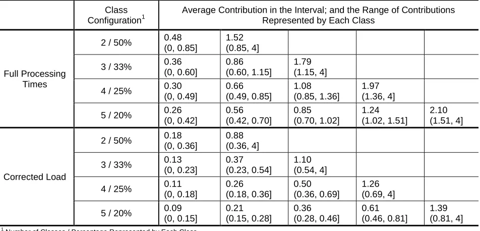
experiments, management does not know the realized processing times (which follow a 2-Erlang distribution) but uses a rough-cut estimate (e.g. small, medium and large for three classes). In doing so, we will assess the robustness of our results to uncertainty in processing time estimates. Table 1 summarizes the classes and the range of workload contributions represented by each class for the full processing time and the corrected load.

[Take in Table 1]

The ranges of contribution for each class were deliberately chosen such that each range would represent an equal percentage of the load contributions. These ranges and the average contribution in each range could be determined analytically for the full processing times. As the corrected load divides these processing times by the routing position resulting from another stochastic process, the ranges for the corrected load contributions have been determined numerically. Of course, in practice, classes will not be determined this exactly, but additional experiments have shown that our results are highly robust to the choice of range.

4.2 The Due Date Determination Procedure

A due date is determined when a job arrives. In addition to our new approach to setting planned release dates (as outlined in Section 3.1), we also include the approach presented in Land (2009) – see Section 2.1.1 – as a benchmark. Both rules apply the same method for setting allowances for the operation throughput times and the external allowance, as identified in Section 2.1.2 and 2.1.3 above. They differ in the way that the pool waiting time and, consequently, the planned release date is estimated.

As in previous research, the time buckets for determining the allowances for the operation throughput times are set to 1 time unit (e.g. Thürer et al., 2013 and 2014a). The external allowance was set through preliminary simulation experiments such that the average of the quoted delivery lead time is 30 time units for all experiments. The quoted delivery lead time is defined as the customer due date minus the time when the job was received.

4.3 Order Release Control

13

according to LUMS COR (see Section 2.2); and (ii) integrated Workload Control, where the periodic release decision is taken as part of the due date setting procedure and jobs are released on their calculated planned release dates without further review. The time interval between releases for the periodic part of order release is set to 4 time units. Eight workload norm levels are applied, ranging from 5 to 12 time units. As a baseline measure, experiments without controlled order release have also been executed, i.e. where jobs are released onto the shop floor immediately upon arrival.

4.4 Priority Dispatching on the Shop Floor

For the due date setting rules to be effective, the dispatching rule applied on the shop floor should be related to the way in which operation due dates are determined. This ensures that capacity control takes place, i.e. that capacity is used as planned (see, e.g. Bertrand 1983a). Therefore, the job with the earliest operation due date (as calculated by the due date setting procedure) is chosen from the queue in front of a station.

4.5 Experimental Design Factors and Performance Measures

The performance of Workload Control based on one decision level will be compared with the use of Workload Control based on two decision levels. Two different versions of Workload Control (WLC) based on two decision levels will be simulated to compare our new planned release date calculation (Section 3.1) with the calculation proposed in Land (2009), as specified in Section 2.1.1. Thus, in total, three approaches – as summarized in Table 1 – will be used: two-level WLC Land, two-two-level WLC, and integrated (single-two-level) WLC. Eight workload norm levels and five levels of classes for processing time estimates (deterministic and stochastic with 5, 4, 3 and 2 classes) are considered for each approach, resulting in an experimental design with 120 cells, where each cell is replicated 100 times. Results are collected over 10,000 time units following a warm-up period of 3,000 time units. These parameters allow us to obtain stable results while keeping the simulation run time to a reasonable level.

[Take in Table 2]

14

standard deviation of lateness. The average lead time is used as the main indicator of the workload balancing capabilities of the approaches being tested. It also reflects the average lateness of jobs,which can be derived directly from this measure and is equal to the average of the realized lead time minus the average of the quoted delivery lead time (which is 30 time units across all experiments). The main indicators of delivery performance are the percentage of tardy jobs and the mean tardiness, which are influenced by both the average lateness and the dispersion of lateness across jobs, as measured by the standard deviation of lateness. In addition to these four main performance measures, we also measure the average shop floor throughput time as an instrumental performance variable. While the overall lead time includes the time that a job waits in the pool prior to release, the shop floor throughput time only measures the time after release to the shop floor. According to Little’s law (Little, 1961), the shop floor throughput time is linked directly to the level of work-in-process. All of these performance measures are job related. This is justified by the fact that the throughput of work (and thus the major shop related performance measure) is kept equal across experiments to ensure comparability.

5. Results

Statistical analyses of our results were conducted using an ANOVA based on a block design. The different approaches to Workload Control and the workload norm level are both blocking factors since each approach to Workload Control and each norm level can be considered a different system. Thus, ANOVA was restricted to the main effects of the three experimental factors considered in this study. All were shown to be statistically significant except the norm level factor for the lead time results. The significance of the differences between the outcomes of individual experiments has also been verified by paired t-tests, which comply with the use of common random number streams to reduce variation across experiments. Whenever we discuss a difference in outcomes between two experiments, the significance can be proven by a paired t-test at a level of 97.5%.

15

5.1 Performance Assessment under Deterministic Processing Times

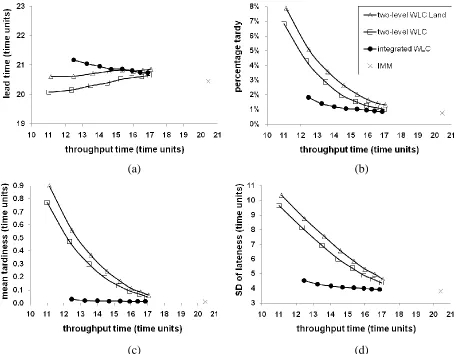
Figures 1a to 1d present our results under deterministic processing times for the lead time, the percentage tardy, the mean tardiness, and the standard deviation of lateness over the throughput time results, respectively. The results are presented in the form of performance curves, where the left-hand starting point of each curve represents the tightest workload norm level (5 time units). The workload norm increases step-wise by moving from left to right, with each data point representing one norm level (from 5 to 12 time units); loosening the norms increases the workload levels and, as a result, the throughput times on the shop floor become longer. In addition, the result obtained with IMMediate release (IMM) is shown as a single point labeled “X”. It is located to the right of the curves as it leads to the highest level of throughput times on the shop floor.

[Take in Figure 1]

16

5.1.1 Performance Analysis: Two-Level WLC vs. Integrated WLC

Both two-level WLC and integrated WLC use the same method for calculating planned release dates. This method schedules the release of jobs into a release interval that should allow for their release on the planned release date. However, under two-level WLC, the planned release date only determines the sequence in which jobs are considered for release. A job is only released when it actually fits the norm at this moment in time. A minor deviation from the schedule may prevent the release of a job on its planned release date. If a job is not released on its planned release date, it may become difficult to fit within the norm again. This can increase the size of the deviation between the planned and actually realized release date, especially for jobs with large corrected processing times, because:

(i) The average capacity available at each station per release interval – measured in corrected processing times – is only 4 time units divided by 2.67, i.e. the average position of a station in the routing of jobs; and,

(ii) LUMS COR releases all of the work that fits within the norm each release interval, even though a large job with an earlier planned release date may be left waiting because it does not fit within the norm. The released jobs replenish the load back up to the norm level and may then block the release of the large job at the next release interval, particularly in periods when many jobs arrive to the system.

To illustrate the above effect, we recorded the properties of all tardy jobs for two-level WLC and for integrated WLC. First, the scatter plots for job lateness versus the maximum corrected processing time across all operations in the routing of a job are given for two-level WLC in Figures 2a to 2c at a norm level of 6, 8 and 10 time units, respectively. Each scatter plot also gives the frequency distribution in the form of a histogram.

[Take in Figure 2]

17

same scatter plots for integrated WLC – see Figures 3a to 3c – demonstrate that the extent of tardiness can be controlled if jobs are released on their planned release dates.

[Take in Figure 3]

5.2 Robustness of Results: Simplifying the Need for Processing Time Estimates

From the results in Section 5.1, it can be concluded that: (i) our new approach to estimating planned release dates enhances performance compared to the existing approach from the literature (two-level WLC vs. two-level WLC Land) across all measures considered in this study; and, (ii) integrated (single-level) WLC outperforms two-level WLC on tardiness performance. But both of these conclusions rest on the assumption that processing times are known during the planning process; i.e. deterministic. This is often not realizable in practice, e.g. due to the high-variety production environment typical of job shops and/or the high investment costs required to achieve high levels of accuracy. Therefore, additional experiments have been conducted in which the need for processing time estimations is simplified by grouping processing times into classes (i.e. processing times are stochastic), as described in Section 4.1.1. Estimates represent a certain range of load contributions, rounded to the estimated average in that range, rather than representing the exact workload contribution of a job. For example, with three classes, a manager need only estimate whether a processing time is small, medium or large.

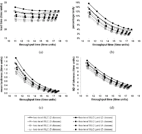
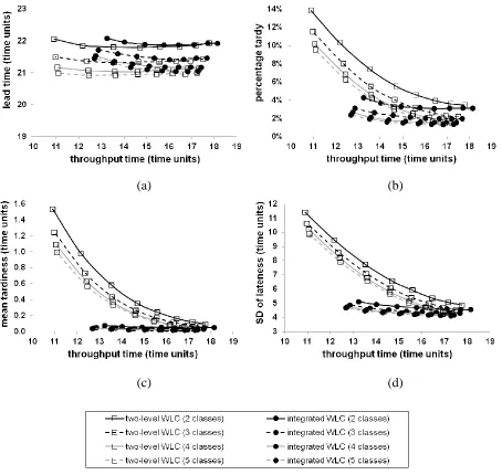
The resulting performance curves for 2, 3, 4 and 5 classes are presented in Figure 4 and Figure 5. Figure 4 presents the results for two-level WLC and two-level WLC Land. Meanwhile, Figure 5 presents the results for two-level WLC and one-level WLC. The results show the expected decreasing marginal effect, e.g. the improvement from 4 to 5 classes is smaller than the improvement from 2 to 3 classes. Most importantly, the results confirm that the performance effects observed in Section 5.1 are robust to uncertainty in processing time estimates.

[Take in Figure 4 & Figure 5] 6. Conclusion

18

typically assumed the immediate release of jobs or used a constant allowance for the pool waiting time. This limits the applicability of due date setting rules previously presented in the literature. In response, this study has developed a new approach to setting planned release dates for integration into Workload Control’s due date setting procedure and demonstrated its effectiveness through simulation. Our approach to estimating planned release dates is unique in that it anticipates Workload Control’s load-limiting order release decision as part of the due date setting procedure. This means that a second independent release decision becomes superfluous. Making the release decision an integral part of the due date setting procedure – by actually releasing all jobs on their planned release dates without further review – means that deviations between planned and realized release dates are avoided. Our analysis revealed that these deviations are a major cause of tardiness for systems with two independent control levels. As a result, for a throughput time reduction of 35% compared to immediate release, 50% fewer tardy jobs and a mean tardiness reduction of more than 90% could be observed for integrated (single-level) Workload Control compared to two-level Workload Control. These results make a compelling argument for a paradigm shift in the literature away from treating due date setting and order release control as two independent decision levels.

6.1 Limitations and Future Research Directions

This research has demonstrated that deviations between the planned release date used to determine the delivery time allowance and the actual realized release date are a major cause of tardiness. These deviations can be avoided if the release decision is anticipated when due dates are set and jobs are released on their planned release dates. This finding questions a fundamental assumption in the literature on production planning and control, i.e. that due date setting and order release are two independent decision levels, where the former precedes the latter. As a consequence, this study calls for a paradigm shift to recognize the potential of the release decision being an integral part of the due date setting procedure.

19

adjustments to ‘catch-up’ with the plan. This may make performance improvements for integrated Workload Control less striking or may even re-balance results in favor of two-level Workload Control. Future research is therefore required to assess whether integrated Workload Control also maintains its advantage when capacity control is exercised.

Finally, another important avenue for future research concerns Advanced Planning and Scheduling (APS) systems (see, e.g. Stadtler & Kilger, 2005). One of the key features of an APS system is Finite Capacity Scheduling, a module that is designed to overcome the weaknesses of Material Requirements Planning (MRP) logic. Similar to our approach, an APS system integrates decision-making, but it is intended for large-scale production environments. Our study may provide an important search direction for extending the applicability of APS systems to smaller scale, complex job shop environments.

References

Ahmed, I., and Fisher, W.W., 1992, Due date assignment, job order release and sequencing interaction in job shop scheduling, Decision Sciences, 23, 633-647.

Bechte, W., 1994, Load-oriented manufacturing control just-in-time production for job shops, Production Planning & Control, 5, 3, 292 – 307.

Bertrand, J.W.M, 1983a, The use of workload information to control job lateness in controlled and uncontrolled release production systems, Journal of Operations Management, 3, 2, 79-92.

Bertrand, J.W.M, 1983b, The effect of workload dependent due-dates on job-shop performance,

Management Science, 29, 7, 799-816.

Bertrand, J.W.M., and Wortmann, J.C., 1981, Production control and information systems for

component-manufacturing shops, Elsevier Scientific Publishing Company, Amsterdam.

Bergamaschi, D., Cigolini, R., Perona, M., and Portioli, A., 1997, Order review and release strategies in a job shop environment: A review and a classification, International Journal of Production Research, 35, 2, 399-420.

Cheng, T.C.E., and Gupta, M.C., 1989, Survey of scheduling research involving due date determination decisions, European Journal of Operational Research, 38, 156-166.

Cigolini, R., and Portioli-Staudacher, A., 2002, An experimental investigation on workload limiting methods with ORR policies in a job shop environment, Production Planning & Control, 13, 7, 602– 613.

Enns, S.T., 1995a, An integrated system for controlling shop loading and work flow, International

20

Enns, S. T., 1995b, A dynamic forecasting model for job shop flow time prediction and tardiness control,

International Journal Production Research, 33, 5, 1295-1312.

Fredendall, L.D., Ojha, D., and Patterson, J.W., 2010, Concerning the theory of workload control,

European Journal of Operational Research, 201, 1, 99-111.

Hendry, L.C., and Kingsman, B.G., 1991, A decision support system for job release in make to order companies, International Journal of Operations & Production Management, 11, 6-16.

Hendry, L. C., Kingsman, B. G., and Cheung, P., 1998, The effect of workload control (WLC) on performance in make-to-order companies, Journal of Operations Management, 16, 1, 63-75.

Hendry, L.C., Huang, Y., and Stevenson, M., 2013, Workload control: Successful implementation taking a contingency-based view of production planning & control, International Journal of Operations &

Production Management, 33, 1, 69-103.

Hopp, W.J., and Sturgis, M.L.R., 2000, Quoting manufacturing due dates subject to a service level constraint, IIE Transactions, 32, 771-784.

Kanet, J.J., 1988, Load-limited order release in job shop scheduling systems, Journal of Operations

Management, 7, 3, 44-58.

Kingsman, B.G., Tatsiopoulos, I.P., and Hendry, L.C., 1989, A Structural Methodology for Managing Manufacturing Lead Times in Make-to-Order Companies, European Journal of Operational Research, 40, 196–209.

Kingsman, B.G., 2000, Modelling input-output workload control for dynamic capacity planning in production planning systems, International Journal of Production Economics, 68, 1, 73-93.

Kingsman, B.G., and Hendry, L.C., 2002, The relative contributions of input and output controls on the performance of a workload control system in Make-To-Order companies, Production Planning &

Control, 13, 7, 579-590.

Land, M.J., 2009, Cobacabana (control of balance by card-based navigation): A card-based system for job shop control, International Journal of Production Economics, 117, 97-103

Land, M.J., and Gaalman, G.J.C, 1996, Workload control concepts in job shops: A critical assessment,

International Journal of Production Economics, 46-47, 535-538.

Land, M.J., and Gaalman, G.J.C., 1998, The performance of workload control concepts in job shops: Improving the release method, International Journal of Production Economics, 56-57, 347-364.

Little, J., 1961, A proof of the theorem L = λW, Operations Research, 8, 383-387.

Lödding, H., 2013, Handbook of Manufacturing Control: Fundamentals, Description, Configuration, Springer: Heidelberg

Melnyk, S.A., and Ragatz, G.L., 1989, Order review/release: research issues and perspectives,

21

Moses, S., Grant, H., Gruenwald, L., and Pulat, S., 2004, Real-time due-date promising by build-to-order environments, International Journal of Production Research, 42-20, 4353-4375.

Nyhuis, P., and Wiendahl, H.P., 2009, Fundamentals of Production Logistics: Theory, Tools and

Applications, Springer: Heidelberg.

Oosterman, B., Land, M.J., and Gaalman, G., 2000, The influence of shop characteristics on workload control, International Journal of Production Economics, 68, 1, 107-119.

Ragatz, G.L., and Mabert, V.A., 1984, A Simulation Analysis of Due Date Assignment Rules, Journal of

Operations Management, 5, 1, 27-39.

Stadtler, H., and Kilger, C., 2005, Supply chain management and advanced planning: concepts, models

software and case studies, Springer, Berlin.

Stevenson, M., Hendry, L.C., and Kingsman, B.G., 2005, A review of production planning and control: The applicability of key concepts to the make to order industry, International Journal of Production

Research, 43, 5, 869-898.

Thürer, M., Stevenson, M., Silva, C., Land, M.J., and Fredendall, L.D., 2012, Workload control (WLC) and order release: A lean solution for make-to-order companies, Production & Operations Management, 21, 5, 939-953.

Thürer, M., Stevenson, M., Silva, C., & Land, M.J., 2013, Towards an integrated Workload Control (WLC) concept: The performance of due date setting rules in job shops with contingent orders, International Journal of Production Research, 51, 15, 4502-4516.

Thürer, M., Stevenson, M., Silva, C., Land, M.J., Fredendall, L.D., and Melnyk, S.A., 2014a, Lean control for make-to-order companies: Integrating customer enquiry management and order release, Production & Operations Management, 23, 3, 463-476.

Thürer, M., Land, M.J., and Stevenson, M., 2014b, Card-Based Workload Control for Job Shops: Improving COBACABANA, International Journal of Production Economics, 147, 180-188.

Thürer, M., Land, M.J., Stevenson, M., and Fredendall, L.D., 2016, Card-Based Delivery Date Promising in High-Variety Manufacturing with Order Release Control, International Journal of Production

Economics; 172, 19-30.

Vig, M.M., and Dooley, K.J., 1993, Mixing static and dynamic flow time estimates for due-date assignment, Journal of Operations Management, 11, 67-79.

Wiendahl, H.P., Gläßner, J., and Petermann, D., 1992, Application of load-oriented manufacturing control in industry, Production Planning & Control, 3, 2, 118–129.

Wisner, J. D., 1995, A review of the order release policy research, International Journal of Operations &

Production Management, 15, 6, 25-40.

22

Zäpfel, G. and Missbauer, H., 1993, New concepts for production planning and control, European

23

Table 1: Definition of the Different Processing Time Classes used in this Study

Class Configuration1

Average Contribution in the Interval; and the Range of Contributions Represented by Each Class

Full Processing Times

2 / 50% 0.48 (0, 0.85]

1.52 (0.85, 4]

3 / 33% 0.36 (0, 0.60]

0.86 (0.60, 1.15]

1.79 (1.15, 4]

4 / 25% 0.30 (0, 0.49] 0.66 (0.49, 0.85] 1.08 (0.85, 1.36] 1.97 (1.36, 4]

5 / 20% 0.26 (0, 0.42] 0.56 (0.42, 0.70] 0.85 (0.70, 1.02] 1.24 (1.02, 1.51] 2.10 (1.51, 4] Corrected Load

2 / 50% 0.18 (0, 0.36]

0.88 (0.36, 4]

3 / 33% 0.13 (0, 0.23]

0.37 (0.23, 0.54]

1.10 (0.54, 4]

4 / 25% 0.11 (0, 0.18] 0.26 (0.18, 0.36] 0.50 (0.36, 0.69] 1.26 (0.69, 4]

5 / 20% 0.09 (0, 0.15] 0.21 (0.15, 0.28] 0.36 (0.28, 0.46] 0.61 (0.46, 0.81] 1.39 (0.81, 4] 1

Number of Classes / Percentage Represented by Each Class

Table 2: Summary of the Different Approaches to Workload Control Applied in this Study

Workload Control

(WLC) Approach

Calculation of Planned Release Dates during the Due Date

Setting Procedure

Order Release

Periodic Element Continuous Element

Two-Level WLC Land

The planned release date is calculated based on the maximum of the load waiting to be released to a station across the stations in the routing of a

job; based on Land (2009).

The release decision is taken independently at order release;

jobs are released up to the workload norm.

All equal; jobs are pulled onto the shop

floor if a station is starving in-between

periodic reviews Two-Level

WLC

The planned release date is determined by forward finite loading, fitting the projected released workload into the

workload norms.

The release decision is taken independently at order release;

jobs are released up to the workload norm.

Integrated WLC

The planned release date is determined by forward finite loading, fitting the projected released workload into the

workload norms.

The release decision is anticipated when due dates are set; jobs are released on their planned release date, as

24

(a) (b)

(c) (d)

Figure 1: Performance Comparison for Deterministic Processing Times: (a) Lead Time; (b) Percentage Tardy; (c) Mean Tardiness; and, (d) Standard Deviation of Lateness over the Shop

25

(a) – Norm 6 (b) – Norm 8 (c) – Norm 10

Figure 2: Scatter Plot of Tardy Jobs Showing the Relationship between the Maximum Corrected Processing Time in the Routing of a Job and Lateness for Two-Level WLC

(a) – Norm 6 (b) – Norm 8 (c) – Norm 10

Figure 3: Scatter Plot of Tardy Jobs Showing the Relationship between the Maximum Corrected Processing Time in the Routing of a Job and Lateness for Integrated WLC

0 1 2 3 4

maximum corrected processing time (time units) 0 25 50 75 100 125 150 175 200 la te n e s s ( ti m e u n it s )

0 1 2 3 4

maximum corrected processing time (time units) 0 25 50 75 100 125 150 175 200 la te n e s s ( ti m e u n it s )

0 1 2 3 4

maximum corrected processing time (time units) 0 25 50 75 100 125 150 175 200 la te n e s s ( ti m e u n it s )

0 1 2 3 4

maximum corrected processing time (time units) 0 25 50 75 100 125 150 175 200 la te n e s s ( ti m e u n it s )

0 1 2 3 4

maximum corrected processing time (time units) 0 25 50 75 100 125 150 175 200 la te n e s s ( ti m e u n it s )

0 1 2 3 4

26

(a) (b)

(c) (d)

Figure 4: Performance Comparison for Simplified Processing Time Estimations (Two-level WLC vs. Two-level WLC Land): (a) Lead Time; (b) Percentage Tardy; (c) Mean Tardiness; and, (d)

27

(a) (b)

(c) (d)

Figure 5: Performance Comparison for Simplified Processing Time Estimations (Two-level WLC vs. Integrated WLC): (a) Lead Time; (b) Percentage Tardy; (c) Mean Tardiness; and, (d)