Adaptive optimization for OpenCL programs on embedded heterogeneous systems

Adaptive Optimization for OpenCL Programs

on Embedded Heterogeneous Systems

Ben Taylor, Vicent Sanz Marco, Zheng Wang

{b.d.taylor, v.sanzmarco, z.wang}@lancaster.ac.uk

Abstract

Heterogeneous multi-core architectures consisting of CPUs and GPUs are commonplace in today’s embedded systems. These architectures offer potential for energy efficient computing if the application task is mapped to the right core. Realizing such potential is challenging due to the complex and evolving nature of hardware and applications. This paper presents an automatic approach to map OPENCL kernels onto heterogeneous multi-cores for a given optimization criterion – whether it is faster runtime, lower energy consumption or a trade-off between them. This is achieved by developing a machine learning based approach to predict which processor to use to run the OPENCL kernel and the host program, and at what frequency the processor should operate. Instead of hand-tuning a model for each optimization metric, we use machine learning to develop a unified framework that first automatically learns the optimization heuristic for each metric off-line, then uses the learned knowledge to schedule OPENCL kernels at runtime based on code and runtime information of the program. We apply our approach to a set of representative OPENCL benchmarks and evaluate it on an ARM big.LITTLE mobile platform. Our approach achieves over 93% of the performance delivered by a perfect predictor. We obtain, on average, 1.2x, 1.6x, and 1.8x improvement respectively for runtime, energy consumption and the energy delay product when compared to a comparative heterogeneous-aware OPENCL task mapping scheme.

Keywords Heterogeneous Multi-cores, Predictive Modeling,

En-ergy Efficiency, OpenCL

1.

Introduction

Embedded systems with heterogeneous multi-cores are common-place. These systems offer the potential of energy efficient comput-ing via diverse processcomput-ing units specially tuned for a certain class of workloads and for power or performance. While promising, to unlock the potential of such systems, software must adapt to the variety of processors, knowing what type of processors to use and at what frequency the processor should operate.

∗_{Corresponding author: Zheng Wang ([email protected]).}

OPENCL has emerged as a standard programming model for heterogeneous systems. It allows the same code to be executed across a variety of processors including CPUs, GPUs and DSPs. While OPENCL provides functional portability, its performance often varies across different processing units [13, 19, 26]. Therefore, there is a need to determine where and how to map a OPENCL task to best utilize the underlying heterogeneous hardware resources.

In this paper, we tackle the issue of OPENCL task mapping across heterogeneous CPUs and GPUs for multiple optimization criteria. Although task scheduling is a heavily studied area [3, 11, 34, 35], heterogeneous task mapping is made more complex by the different runtime and energy characteristics an OPENCL kernel will experience on different processing units [9, 28, 30]. While manually task mapping may be possible in certain domains [2, 4], it is not the general case as the decision will depend on: the application itself, the program input, underlying hardware, and optimization criteria. Given that embedded systems are becoming increasingly diverse with ever-changing hardware and software, finding the right mapping for a single application may have to be repeated many times throughout its lifetime, hence, making automatic approaches attractive.

This paper presents a novel compiler-based approach to map and schedule OPENCL tasks across embedded heterogeneous computing units. We do so by employing machine learning techniques to automatically construct predictors to determine at runtime the optimal processor configuration – which processing units and clock frequencies to use to run the given OPENCL driver program and kernel function, taking into consideration the optimization criterion – whether it is faster response time, lower energy consumption or a trade-off between them. Our predictors are first trainedoff-line. Then, using code and data features extracted from the compiler intermediate representations (IR), the models predict the optimal processor configuration for anew,unseenprogram, depending on what we want to optimize for. We show that our unified machine learning based framework can automatically derive high-quality optimization heuristics across different optimization metrics, despite the optimal configurations changing from one metric to the other. Our approach avoids the pitfalls of using a hard-wired heuristics that require human modification every time the optimization criterion or hardware changes.

We apply our approach to 15 OPENCL benchmarks and evaluate them on a representative big.LITTLE mobile platform, using three metrics: runtime, energy consumption and the energy delay product. We compare it to a comparative machine learning based mapping scheme [13]. We show that our approach delivers, on average, over 1.2x improvement across all benchmarks.

This paper makes the following two main contributions: • We develop a unified machine learning based framework for

•We show that our automatic approach constantly outperforms comparative work across all evaluation metrics.

2.

Related Work

Our work lies at the intersection of numerous areas: GPU perfor-mance optimization, GPU task scheduling, predictive modeling and energy optimization.

GPU Performance Optimization There is an extensive body of

work looking at GPU performance optimization through the use of compilation and runtime techniques [22, 31, 38]. Most prior work in the field uses analytical models to determine optimization strategies. contrast, our work employs machine learning to automatically construct models for different optimization goals. Prior studies show that portable mapping techniques are important, program performance depends on the underlying hardware [19, 26]. Our work is among attempts to create portable mapping techniques.

GPU Task Scheduling Numerous approaches have been proposed

to map OPENCL or CUDA kernels on heterogeneous computing devices. Some of the prior work uses profile runs to partition work across the CPU and the GPU [1, 13, 20, 23]. In contrast to these works, our approach does not rely on profiling information, therefore, has less runtime overhead. Other work considers code and data transformations for CPU/GPU architectures [21, 27], GPU task pre-emption [6], and multi-task scheduling [10, 14–16, 22, 43]. These prior works primarily target performance optimization, while this work aims to build a portable approach for arbitrary optimization goals. Moreover, existing approaches on multi-task scheduling are orthogonal to our work.

Predictive Modeling Machine learning based predictive modeling

is emerging as a powerful technique for optimizing parallel pro-grams [28, 29, 33, 37, 39–41]. Its great advantage is its ability to adapt to changing platforms as it has no a prior assumptions about their behavior. The work presented by Greweet al.is the nearest work [13, 42], which builds a decision tree model to predict where (CPU or GPU) to run a given OPENCL kernel. Our approach differs from this work in two aspects. Firstly, our approach can adapt to dif-ferent optimization goals while [13] only targets runtime. Secondly, our approach considers the clock frequency of the processors while [13] does not.

Energy Optimization How to effectively exploit heterogeneous

architectures for energy efficient computing is a heavily studied area. Some of the recent examples in the area include: how to distribute workloads across CPUs and GPUs [25] and MPSoCs [4], power modeling for GPGPUs [24], and energy aware iterative compila-tion [7, 12] etc. Unlike these approaches which all use analytic models or hard-wired heuristics to perform optimization for a spe-cific goal, we develop a portable method that can automatically re-target for any optimization metric. Our approach shares the same spirit as the work presented by Renet al.[32], we both use machine learning to build predictive models for energy optimization. How-ever, we target optimizing OPENCL programs on heterogeneous systems, while [32] focuses on scheduling mobile web browsing processes on CPUs.

3.

Background

3.1 Problem Definition

Scope This work aims to develop a runtime system that can adapt

to arbitrary optimization goals for OPENCL kernel mapping. An OPENCL program typically consists of two parts, a kernel program (which might contain several OPENCL kernel functions) to run on an OPENCL-compatible device (in our case a CPU or GPU), and a driver (or host) program to run on the general purpose CPU

to offload the kernel computation. OPENCL kernel functions are compiled at runtime on the host CPU and sent to execute on the compatible device. This work is concerned with determining the best processor configuration – that is – which processor to run the driver program and the kernel, and at what clock frequency the processing units should operate.

Notation Our configuration notation is HostDev.b/L,f req −

KernelDev.b/L, wherebandLstands for big and little CPU/GPU

respectively. For example, notation,CP UL,800M hz−GP Ub, means

running the host program on the little CPU at 800Mhz and the kernel on the big GPU. It is to note that we found that using the default frequency to run the OPENCL kernel gives the best performance, so we do not configure the clock frequency for running the kernel.

Optimization Metrics Unlike prior work [13], we do not just

develop a method to optimize runtime. Instead, we want to develop a methodology that can be used for any optimization goal. For the purpose of evaluation, we target threelower is bettermetrics: (a)runtime, which aims to execute the kernel function as fast as possible; (b)energy consumption, which aims to use as little energy as possible; and (c)energy delay product (EDP), calculated as energy×runtime, which aims to find a balance between both energy consumption and performance.

Hardware platform Our work targets the ARM big.LITTLE

archi-tecture. These platforms couple a energy-tuned processor (LITTLE) with a faster and more power-hungry processor (big), some also come with a GPU which can be used for general purpose comput-ing. The uniqueness of each processing unit allows for much more energy efficient computing when utilized to its full potential. Our work is evaluated on an Odroid-Xu3 embedded development board. We chose this platform as it is: representative of ARM big.LITTLE mobile architectures, provides us with an OPENCL implementation for both the CPU and GPU, and allows us to extract real-time energy readings using the on-board energy sensors. The architecture used in the Odroid system is used in multiple mobile devices such as the Samsung Galaxy S5.

3.2 Motivating Example

Consider scheduling four OPENCL kernels from the Rodinia bench-mark suite on an ARM big.LITTLE platform with heterogeneous processing units. These kernels can be run on either of the heteroge-neous CPU clusters, a Cortex-A15 processor (big) and a Cortex-A7 processor (little), or the Mali-T628 GPU. The OPENCL libraries recognise the Mali-T628 as two separate GPUs, one containing 4 cores (big), the other containing two (little).

Table 1 lists the best processor configurations for each of the three metrics considered in this work. To obtain the optimum processor configurations we performed an exhaustive search across all configurations, and monitored the energy consumption and runtime of each. We then calculated the processor configuration which produced the minimum value (as each metric is lower-is-better) for each metric and kernel combination.

Figure 1 compares the potential improvement of each kernel and metric over a baseline that runs all kernels on the big GPU,

CP UB,2.0Ghz−GP Ub. For runtime, the baseline performs well for

BFS_1andNearest Neighbor, but a speed-up of 51% and 80%

Table 1: The best configuration which optimizes for each of the metrics: Energy Consumption, Runtime, and EDP.

Kernel Energy Consumption Runtime EDP

BFS_1 CP UL,800M hz−GP Ub CP UL,1.4Ghz−GP Ub CP UL,1.2Ghz−GP Ub

find_index CP UL,800M hz−CP Ul CP UB,2.0Ghz−CP Ub CP UB,1.6Ghz−CP Ub

Nearest Neighbor CP UL,1.0Ghz−GP Ul CP UB,2.0Ghz−GP Ub CP UL,1.4Ghz−GP Ul

lud_diagonal CP UL,800M hz−CP Ul CP UB,2.0Ghz−CP Ub CP UL,1.2Ghz−CP Ul

B F S _ 1 N e a r e s t N e i g h b o r f i n d _ i n d e x l u d _ d i a g o n a l

0

2 0 4 0 6 0 8 0 1 0 0

Im

pr

ov

em

en

t o

ve

r b

ig

-G

PU

o

nl

y

(%

)

R u n t i m e

E n e r g y C o n s u m p t i o n E D P

Figure 1: The percentage decrease (higher is better) of different metrics achieved when choosing the optimum configuration. The baseline is offloading each kernel to the big GPU,CP UB,2.0Ghz−

GP Ub.

B F S _ 1 N e a r e s t N e i g h b o r f i n d _ i n d e x _ k e r n e l l u d _ d i a g o n a l

0

2 0 4 0 6 0 8 0 1 0 0

Im

pr

ov

em

en

t o

ve

r

BF

S_

1-ED

P

op

tim

um

(%

) R u n t i m e E n e r g y C o n s u m p t i o n

E D P

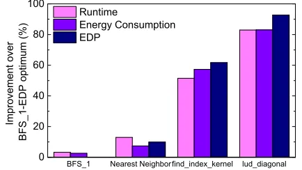
Figure 2: Available room for improvement when using the opti-mum configuration found for BFS_1when optimizing for EDP,

CP UL,1.2Ghz−GP Ub. This diagram shows that the best

configu-ration varies across metrics and programs.

Figure 2 normalizes the best available performance of each met-ric forfind_index,lud_diagonal, andNearest Neighborto the performance achieved by using the best configuration found for

BFS_1, when optimizing for EDP (BFS_1-EDP). It shows that the

best configuration also changes from one kernel to another; in other words no one configuration can be used to optimize for all kernels and all metrics. Overall, the best configuration forBFS_1-EDP pro-vides a near optimal choice across all metrics forBFS_1.Nearest

Neighboralso achieves near optimum results across all metrics

for this configuration; although, a improvement of 13%, 7%, and 9% can still be achieved for runtime, energy consumption and EDP respectively. Kernelsfind_indexandlud_diagonalachieve far from optimal results under this configuration. The best configuration is able to give an improvement between 51% and 92% (average of 71%) for all metrics. Therefore, finding an optimal configuration for one kernel and applying it to all others is likely to miss significant op-timization opportunities. This example demonstrates that choosing the right processor setting has a significant impact on the resultant performance and energy consumption, and the optimal configuration must be determined on a per-kernel and per-optimization-goal basis. Attempting to find the optimum configuration through means of an exhaustive search would be ineffective, the overhead involved would be far bigger then the potential benefits. Classical

hand-Feature Extraction

feature values Predictor

processor config. Scheduling

kernels

Figure 3: Overview of our approach.

written heuristics are not ideal either, as they are not only complex to develop, but are likely to fail due to the variety of programs and evolving OPENCL devices. An alternate approach, and the one we chose to use, is to use machine learning to automatically con-struct predictive models for determining processor configurations, providing minimal runtime and development overhead.

4.

Overall Methodology

Our approach takes anew,unseenOPENCL kernel function and is able to predict the optimum, or near optimum, processor configura-tion. An overview of our approach can be seen in Figure 3, and is described in more detail in Section 5.1.

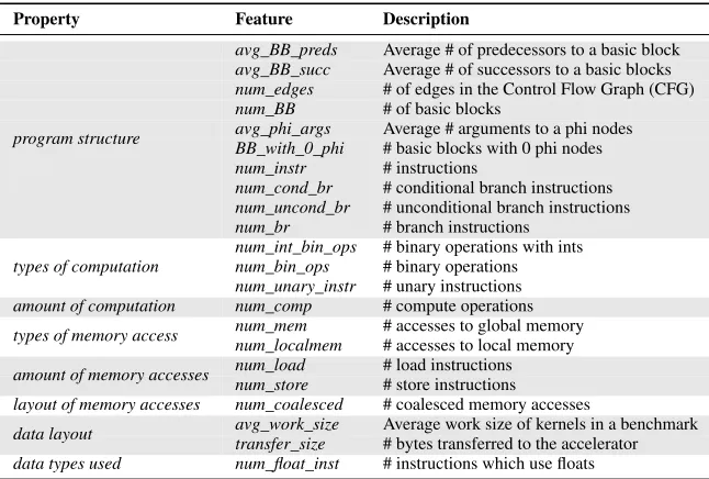
When an OPENCL kernel is launched, our approach will collect a set of information orfeaturesto capture the characteristics of the kernel. As OPENCL is just-in-time compiled, the set of feature values collected by our approach can reflect the program input that is available at runtime. Feature extraction is performed on the LLVM intermediate represenations (IR); we only use code features and do not profile the program. Table 2 presents a full list of all our considered features. After collecting the feature values, a machine learning based predictor (that is trained offline) takes in the feature values and predicts which processor configuration should be used to execute the OPENCL kernel. This prediction includes the choice of host processor and its configuration in conjunction with the choice of accelerator. Finally, when the OPENCL kernel is ready to be offloaded to an accelerator we configure the host processor and offload the kernel to the predicted processor.

5.

Predictive Modelling

Our model for predicting the best processor configuration is com-prised of a set of Support Vector Machines (SVMs) arranged a hi-erarchically, show in Figure 4. Varying degrees of the polynomial kernel is used for each of ourSVMs. We have evaluated a number of alternate modelling techniques, including regression, Naive Bayes, K-Nearest neighbour, decision trees, and artificial neural networks (see also Section 8.2). We choseSVMbecause it gives the best per-formance and can model both linear and non-linear problems. The input to our model is a set of features extracted from the target OPENCL kernel function. The output of our model is a label that in-dicates the optimal processor configuration to the host program and the OPENCL kernel, including the frequency of the host processing unit.

Building and using such a model follows the 3-step process for supervised machine learning: (i) generate training data (ii) train a predictive model (iii) use the predictor, described as follows.

5.1 Model Description

Table 2: Raw features we considered using in this work.

Property Feature Description

avg_BB_preds Average # of predecessors to a basic block avg_BB_succ Average # of successors to a basic blocks num_edges # of edges in the Control Flow Graph (CFG) num_BB # of basic blocks

avg_phi_args Average # arguments to a phi nodes BB_with_0_phi # basic blocks with 0 phi nodes num_instr # instructions

num_cond_br # conditional branch instructions num_uncond_br # unconditional branch instructions program structure

num_br # branch instructions num_int_bin_ops # binary operations with ints num_bin_ops # binary operations types of computation

num_unary_instr # unary instructions amount of computation num_comp # compute operations

num_mem # accesses to global memory types of memory access

num_localmem # accesses to local memory num_load # load instructions amount of memory accesses

num_store # store instructions

layout of memory accesses num_coalesced # coalesced memory accesses

avg_work_size Average work size of kernels in a benchmark data layout

transfer_size # bytes transferred to the accelerator data types used num_float_inst # instructions which use floats

Table 3: Combined features used in this work.

Property Feature Calculated

Ratio of memory access per work size mem_by_work (num_localmem+num_mem) *avg_work_size

Ratio of computation to memory transfer comm-comp_ratio transfer_size/ (num_mem+num_comp)

Ratio of memory access to computation comp-mem_ratio num_comp/num_mem

Percentage of coalesced memory access perc_coal_mem_acc num_coalesced/num_mem

Percentage or memory accesses per instruction mem_acc_per_instr (num_load+num_store) /num_instr

Ratio of transfer size to work size transfer-work_ratio transfer_size/avg_work_size

Initial Kernel on Host Kernel on Accelerator

Accelerator and

host config. Systemconfig.

Accelerator config. Host config. System config. Figure 4: Our model, comprised of 4SVMs. The first (Initial) predicts which type of device to run a kernel. The result then defines which branch we take through our model. Each branch predicts the system configuration for the given kernel. See Section 5.1.

content

Style Rules

Training kernels

Profiling runs

Feature extraction

optimal proc. config.

feature values

L

ea

rn

in

g

A

lg

or

ith

m

Predictive Model

Figure 5: The training process. Our unified machine learning frame-work uses the same procedure to train a hierarchical predictive model for each optimization goal.

Initial The firstSVMin our model, all data which enters our model

passes thisSVMfirst.Initialis used to place each kernel into one of two groups:accelerate-on-hostandaccelerate-off-host, which will be passed to theAccelerator and Host ConfigandAccelerator ConfigSVMsrespectively. Each group requires a different approach to predict the optimum processor configuration for a kernel, hence our use of multiple branches.

Accelerator and Host Config The OPENCL API for our system

recognises both CPUs as one processor, this resulted in us being unable to separate the host and kernel processes. As a result, when a kernel runs on the host it must adopt the same processor set-up

as its host process.Accelerator and Host Configis able to predict the optimum processor configuration while taking the previously mentioned restriction into account. This is the onlySVM in this branch of our predictive model, producing the finalSystem Config

output for this branch.

Accelerator Config Another branch of our predictive model starts

here. Contrary to the previous branch,Accelerator Configpredicts the optimum accelerator configuration only, the optimum host configuration will be predicted byHost Config, which is the next

SVMin this branch.

Host Config As the finalSVMin this branch,Host Configpredicts

the best host configuration. The output of thisSVMandAccelerator Configis then combined to produce the finalSystem Configoutput for this branch of the model.

5.2 Training the Predictor

Our method for training the predictive models is shown in Figure 5. To train a new predictor we first need to find the best processor configuration for each of our training OPENCL kernels, and extract features. We then use this set of data and classification labels to train our predictor model.

Generating Training Data We use leave-one-out-cross validation

the gap of the upper and lower confidence bounds is smaller than 5% under a 95% confidence interval setting. To reduce noise in our performance and energy consumption readings we generate our training data on a unloaded machine, this should not be a problem as we expect model training to be aone-offcost which is carried out at the factory, that is, before a process architecture is released for sale. However, if the hardware configuration changes, i.e. one or more processors are added or removed, new training data will need to generated and the model re-trained. The set of frequencies to be used for generating the training data is decided beforehand. For our hardware platform we chose to use steps of 200Mhz for each processor configuration, e.g. 200Mhz, 400Mhz, up to 2.0Ghz. We exhaustively execute each OPENCL kernel across all of our considered processor configurations, and record the performance and energy consumption of each. Next, we record the best performing processor configuration for each OPENCL kernel and optimization metric, keeping a label of each. Finally, we extract the values of our selected set of features from each OPENCL kernel; our choice of features is described in more detail in Section 5.3.

Building The Model The processor configuration labels, along

with their corresponding feature set, are passed to our supervised learning algorithm. The learning algorithm tries to find a correlation between the feature values and optimal processor configuration labels. The output of our learning algorithm is a version of ourSVM

based model. Because we target three optimization metrics in this paper, we have constructed three predictive models - one for each of our optimization metrics. In our case, the overall training process (which is dominated by training data generation) takes less than a week on a single machine.

Total Training Time The total training time of our model is

comprised of two parts: gathering the training data, and then building the model. Gathering the training data consumes most of the total training time, in this paper it took around 3 days. In comparison actually building the model took a negligible amount of time, less than 1 minute.

5.3 Features

Our predictive models are based exclusively on code features of the target OPENCL kernel. The features are extracted using a pass working on the LLVMIR. Since our goal is to develop aportable, architecture-independent approach, we do not use any hardware-specific features.

We considered a total of 22 candidate raw features (Table 2) in this work. Some features were chosen from our intuition based on factors that can affect kernel mapping e.g.transfer_sizeand

num_float_inst, other features were chosen based on previous

work [13, 26]. Altogether, our candidate features should be able to represent the intrinsic parts of each OPENCL kernel.

Feature Selection In order to build an accurate predictive model

through supervised learning the training sample size typically needs to be at least one order of magnitude greater than the number of features. We currently have 32 OPENCL kernels and 22 features, so we would like to reduce the number of features in use. Our process for feature selection is fully automatic, described as follows. Initially, we reduced our feature count by combining several features to form a set of combined normalized features, shown in Table 3, which are able to carry more information than their parts. Next, we removed any features which carried very similar information as our combined features or their parts, making them redundant. To find which features are closely correlated we constructed a correlation coefficient matrix, which is able to quantify the correlation between any two features. We used Pearson product-moment correlation coefficient. As input, two features are given, a value between +1 and -1 is returned. The closer a coefficient is to +/-1, the stronger the

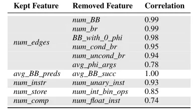
Table 4: Correlations of removed features to the kept features. All correlation values are absolute values.

Kept Feature Removed Feature Correlation

num_BB 0.99

num_br 0.99

BB_with_0_phi 0.98 num_cond_br 0.95 num_uncond_br 0.94 num_edges

avg_phi_args 0.78 avg_BB_preds avg_BB_succ 1.00 num_instr num_unary_inst 0.93 num_store num_int_bin_ops 0.85 num_comp num_float_inst 0.74

Table 5: Features which remained after feature selection.

mem_by_work comm-comp_ratio mem_acc_per_instr comp-mem_ratio perc_coal_mem_acc avg_BB_preds transfer-work_ratio num_edges transfer_size

correlation between the two input features. We removed any feature which had a correlation coefficient (taking the absolute value) greater than 0.75. Table 4 shows all the features which were removed due to a high correlation value with another feature. For example, we can see thatnum_BB is highly correlated tonum_edges, in this case we chose to removenum_BBfrom our feature collection. Our feature selection process results in just 9 features remaining for use, these are listed in Table 5. It is to note that our approach for feature selection is automatic. This means the approach can be applied to other sets of candidate features.

Feature Scaling Before the chosen features can be given to our

predictive model for training they need to be scaled to a common range. We scaled each of our features between the range of 0 and 1. To scale features extracted from anewkernel during runtime deployment we record the maximum and minimum value of each feature before scaling.

5.4 Runtime Deployment

Once we have built and trained our predicted models as described above, we can use them to quickly and efficiently predict the best processor configuration for anynew,unseenOPENCL kernel.

We implemented our approach as an OpenCL library extension, building on standard OPENCL APIs. The kernel code will be trans-lated into LLVMIRwhen the OPENCL APIclBuildProgramis invoked by the host code. Once the kernel function is launched throughclEnqueueNDRangeKernel, our extension extracts and scales all features needed for the predictive model. Given an opti-mization goal our extension will choose the correct predictive model to predict the optimal processor configuration. This prediction is then passed to the runtime library to configure the hardware. It is to note that we use the proprietary OPENCL compiler to compile the kernel for the target hardware. The overhead of extracting features, making predictions, and processor configuration is small, which is included in our experimental results.

6.

Experimental Setup

6.1 Platform and Benchmarks

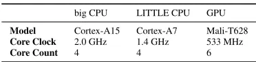
Hardware Our hardware evaluation platform is an Odroid XU3

Table 6: Hardware platform

big CPU LITTLE CPU GPU

Model Cortex-A15 Cortex-A7 Mali-T628

Core Clock 2.0 GHz 1.4 GHz 533 MHz

Core Count 4 4 6

Systems Software Our platform runs Ubuntu 14.04 Linux with a

Heterogeneous Multi-Processing (HMP) scheduler. The scheduler allows us to use the heterogeneous cores at the same time. Our host compiler is gcc v5.4.0, with “-O3" as the compiler option. To use OPENCL on the GPU we use the ARM Mali OPENCL SDK. To use OPENCL on the CPU we use PoCL [18], an OPENCL imple-mentation for CPUs that is based on LLVM. The PoCL compiler automatically applies a set of LLVM-based code transformations to optimize the GPU-tuned OPENCL kernel function for the host CPU.

Benchmarks We used a total of 32 OPENCL kernels from 15

benchmarks. From the Rodinia benchmark suite v2.0.1, we used 22 kernels from 9 benchmarks, and from the Parboil OPENCL benchmark suite, we used 10 kernels from 6 benchmarks. Some benchmarks had to be left out as they were either not compatible with our hardware, or not compatible with our OPENCL compilers.

6.2 Evaluation Methodology

Model Evaluation We useleave-one-outcross-validation to

eval-uate our machine learning model. This means we train our model on 14 benchmarks and apply it to the testing program. We repeat this process 15 times, one for each of the 15 benchmarks. It is a standard evaluation methodology, providing an estimate of the generalization ability of a machine-learning model in predictingunseendata.

Comparisons We compare our approach to another machine

learn-ing based approach which provides a portable mapplearn-ing of OPENCL kernels for heterogeneous systems [13], referred to asPKMhereafter. It is currently the closest work to our own.PKMuses a decision tree to predict whether a given OPENCL program should run on the GPU or the CPU host to achieve the best performance speed-up. We also compare our work to a perfect predictor, referred to as anOraclehereafter. TheOraclepredictor, named after its ability to make prophetic predictions, is able to predict the best possible configuration for all kernels and optimization targets.

Performance Report We profiled each kernel under a processor

configuration multiple times and report thegeometric meanof each metric. To determine how many runs are needed, we calculated the confidence range using a 95% confidence interval and make sure that the difference between the upper and lower confidence bounds is smaller than 5%. To eliminate the impact of outliers, we also reportharmonic means andmedianvalues across kernels and benchmarks. We used the on board energy sensors to measure the entire system. These sensors have been checked against external power measurement instruments and proven to be accurate [17]. To measure the energy consumption, we have developed a lightweight runtime to take readings from the on-board energy sensors at a frequency of 10 samples per second. We then matched the readings against the timestamps of the kernel to calculate the energy consumption.

7.

Experimental Results

In this section, we compare our work againstPKM, showing how our work compares to comparative work. Next, we evaluate our approach against an ideal predictor, anOracle, showing that our approach can deliver over 93% of theOracle’s optimizing capability. Finally, we investigate the impact of different input sizes on our model.

7.1 Overall Performance

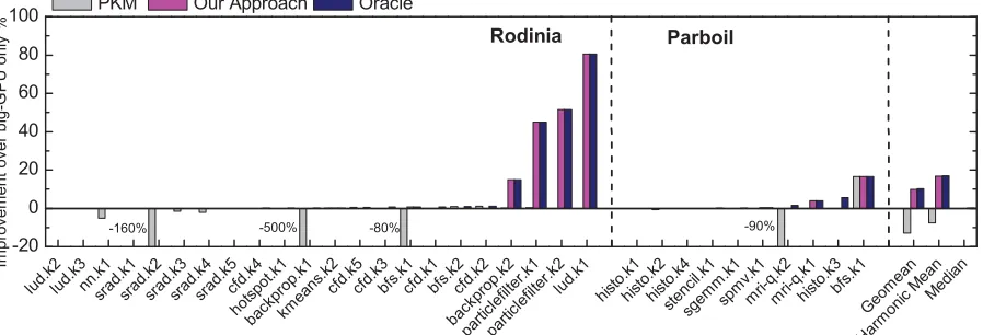
We compare our approach againstPKMon runtime (Figure 6), energy consumption (Figure 7), and EDP (Figure 8). The baseline is to offload all kernels on to the big GPU,CP UB,2.0Ghz −GP Ub.

First, we deeply analyse our results on a per-kernel basis, then we summarize these results on a per-benchmark basis.

Runtime Figure 6 shows the performance achieved by each

method when optimizing for runtime, i.e. when a fast response time is the priority. For this metric, the default method of offloading all kernels on to the big GPU already provides near optimum results for most kernels. This is not a surprising result as the OPENCL benchmarks have been heavily tuned for runtime on GPUs. For this metric,PKMis able to select the correct configuration for most of the kernels, but can lead to significant slowdowns for some. For exam-ple, it gives 1.6x and 5x slowdown forsrad.k1andhotspot.k1

respectively, by predicting the wrong processor to use. Our approach, by contrast, never gives any slow-down in execution time. In fact, by predicting to use the CPU, our approach is able to deliver over 15% (up to 80%) speed-up for some of the kernels which do not benefit from the GPU execution. Overall, our approach gives an average speed-up of 9.4%.

Energy Consumption Figure 7 compares our approach against

PKMwhen optimizing for energy consumption, i.e. when trying to preserve battery life is the main priority. Both methods are able to reduce energy consumption for more than half of the kernels. For this metric, using the power-hungry GPU is not always desired. For some of the kernels,PKMdelivers rather poor energy efficiency performance, consuming up to 8x more energy, because it maps the kernel to run on a device with a much longer execution time than the big GPU. Comparing toPKM, while our approach also gives the wrong prediction for some of the kernels, e.g.mri-q.k2and

histo.k3, the performance degradation is modest (11% and 2%

respectively). We believe the prediction accuracy of our model can be improved by using more examples during training. On average,

PKMachieves a 28% improvement for this metric, which is again outperformed by our approach that gives a 45% improvement. This means that our approach outperformsPKMby a factor of 1.6x when optimizing for energy consumption.

EDP Figure 8 shows the performance achieved by each method when optimizing for EDP, i.e. trying to reduce energy consumption without significantly increasing execution time. Both methods are able to achieve some performance increase over the baseline for EDP. While both approaches are not able to achieve a performance increase every time, our approach limits its performance degradation to -12%, whereasPKM reaches -9.7x for cfd.k5 and -8.1x for

stencil.k1. This huge decrease in EDP can be explained byPKM

predicting these benchmarks to be offloaded to the CPU incorrectly, which gives a significantly longer execution time over the baseline. Overall,PKMfails to deliver any improved performance for EDP (-19%). Our approach, however, is able to give an average performance increase of 32% (up to 96%), with a significant improvement for the majority of benchmarks.PKMis only able to slightly outperform our approach in one instance for EDP optimization; it is caused by our approach incorrectly predicting the host device.

7.2 Comparing with the Oracle

lud. k2

lud. k3

nn.k1_srad.k1_srad.k2_srad.k3_srad.k4_srad.k5cfd.k4 hotspot .k1 backprop. k1 kmeans .k2

cfd.k5cfd.k3bfs.k 1 cfd.k1bfs.k

2 cfd.k2 backprop. k2 parti clefilt er.k1 parti clefilt

er.k2_lud.k1 histo. k1 histo. k2 histo. k4 stenci l.k1 sgem m.k1 spm v.k1 mri-q .k2 mri-q .k1 histo. k3 bfs.k 1 Geom ean Harm onic M

ean Medi an -20 0 20 40 60 80 100 Parboil -90% -80% -500% Im prov em ent ov er b ig -G P U onl y %

PKM Our Approach Oracle

-160%

Rodinia

Figure 6: Optimization for runtime for each kernel. Our approach outperformsPKMand does not slowdown any programs. We achieve, on average, 93.9% of theOracleperformance for this metric.

bac kprop.

k1

kmeans .k2

cfd.k4lud.k3 hotsp ot.k1 bac kprop. k2 parti clefilt er.k1 srad. k3

cfd.k5_srad.k4cfd.k3bfs.k 2 lud.k2bfs.k

1 srad. k1 srad. k2 srad. k5 part iclef ilter.k 2

cfd.k1cfd.k2nn.k1lud.k1 sgemm. k1 stenc il.k1 mri-q .k2 histo. k3 spm v.k1 histo. k2 histo. k4 histo. k1 mri-q .k1 bfs.k 1 Geom ean Harm onic M

ean Medi an -20 0 20 40 60 80 100 -36% -130% -800% Parboil Rodinia Im prov em ent ov er b ig -G P U onl y %

PKM Our Approach Oracle

Figure 7: Optimizing for energy consumption for each kernel. Our approach outperformsPKMand only uses more energy in one kernel compared to the baseline. We achieve, on average, 96.8% of theOracleperformance for this metric.

bac kprop. k1 bac kprop. k2 kmeans .k2

cfd.k4lud.k3

hotsp ot.k1 parti clefilt er.k1 srad. k3 srad. k4

cfd.k5bfs.k

2

cfd.k3lud.k2bfs.k

1 srad. k2 srad. k5 srad. k1 cfd.k1 part iclef ilter.k 2

cfd.k2nn.k1lud.k1

sgemm. k1 stenc il.k1 mri-q .k2 spm v.k1 histo. k3 histo. k2 histo. k4 histo. k1 mri-q .k1 bfs.k 1 Geom ean Harm

onic M

ean Medi an -20 0 20 40 60 80 100 -19% -29% -970% -810% -580% Parboil Rodinia Im prov em ent ov er b ig -G P U onl y %

PKM Our Approach Oracle

Figure 8: Optimization for EDP for each kernel. Our approach outperformsPKMand only leads to a small increase in EDP when compared to the baseline for a few kernels. We achieve, on average, 96.1% of theOracleperformance for this metric.

the performance of our predictive model by increasing the accu-racy of host processor configuration predictions. We suggest that this would be possible through the introduction of more/different features which are capable of characterizing the host program bet-ter than we are currently able. Our model could also be improved through the inclusion of more OPENCL kernels to allow us to better train our models. There could be cases where a model cannot be

trained because of a lack of data, this can be solved by including more, and a wider range, of kernels [8].

7.3 Improvement Per Benchmark

back prop

gaus sian

kmea

ns nw cfd lud hotsp

ot

parti clefilt

er srad bfs nn

sgem m stenc il m ri-q spm v

histo bfs Geom ean Harm onic Mea n Med ian -20 0 20 40 60 80 100

-19% -45% -94%

-371% Im pr ov em en t o ve r bi g-G P U o nl y %

PKM Our Approach Oracle

Rodinia Parboil

Figure 9: Optimization for runtime for each benchmark. Our ap-proach outperformsPKMand does not slowdown any programs. We achieve, on average, 92.6% of theOracleperformance for this metric. back prop gaus sian kmea

ns nw cfd lud hotsp

ot

parti clefilt

er srad bfs nn

sgem m stenc il m ri-q spm v

histo bfs Geom ean Harm onic Mea n Med ian -20 0 20 40 60 80 100 Im pr ov em en t o ve r bi g-G P U o nl y %

PKM Our Approach Oracle

Rodinia Parboil

-555% -42% -36%

Figure 10: Optimizing for energy consumption for each benchmark. Our approach outperformsPKMand only one benchmark consumes more energy compared to the baseline. We achieve, on average, 91.4% of theOracleperformance for this metric.

back prop

gaus sian

kmea

ns nw cfd lud hotsp

ot

parti clefilt

er srad bfs nn

sgem m stenc il m ri-q spm v

histo bfs Geom ean Harm onic Mea n Med ian -20 0 20 40 60 80 100 Im pr ov em en t o ve r bi g-G P U o nl y %

PKM Our Approach Oracle

-5025%

Rodinia Parboil

-373% -29% -811% -71%

Figure 11: Optimization for EDP for each benchmark. Our approach outperformsPKMand only leads to a small increase in EDP when compared to the baseline for a few benchmarks. We achieve, on average, 84.5% of theOracleperformance for this metric. We achieve 92.6%, 91.4%, and 84.5% of theOracle’s optimizing capability for performance, energy consumption, and EDP respec-tively. Comparing on a per-benchmark basis shows our model’s capability to achieve high levels of theOracle’s performance not only for each kernel but for the whole benchmark, i.e. while taking every kernel execution into account.

7.4 Prediction Accuracy

Our predictive model is comprised of 4 SVMs organized in a hierarchical structure (Figure 5, Section 5.1). EachSVMis trained separately on the subset of data which is relevant to it, i.e.SVM Accelerator Configis only trained on the kernels which run best on the accelerator, whereasInitialis trained on all kernels. Overall, our predictive model achieves a high accuracy. The predictive models for performance and energy consumption are able to achieve 100% prediction accuracy. Any reduction in performance when compared to theOracle are due to assumptions about the Host Device’s frequency, that is, some frequencies of the same host are considered as one to help train our model, e.g. kernels with optimum configurations of CP UL,1.2Ghz −CP Ub andCP UL,1.4Ghz −

C -1 C -2 C -3 C -4 C -5 C -6 C -7 C -8 C -9 C -1 0 C -1 1 C -1 2 C -1 3 C -1 4 C -1 5 C -1 6 C -1 7 C -1 8 C -1 9 C -2 0 C -2 1 C -2 2 C -2 3 0 2 4 6 8 10 12 N um be r of K er ne ls (a) Runtime C -1 C -2 C -3 C -4 C -5 C -6 C -7 C -8 C -9 C -1 0 C -1 1 C -1 2 C -1 3 C -1 4 C -1 5 C -1 6 C -1 7 C -1 8 C -1 9 C -2 0 C -2 1 C -2 2 C -2 3 0 2 4 6 8 10 12 N um be r of K er ne ls

(b) Energy consumption

C -1 C -2 C -3 C -4 C -5 C -6 C -7 C -8 C -9 C -1 0 C -1 1 C -1 2 C -1 3 C -1 4 C -1 5 C -1 6 C -1 7 C -1 8 C -1 9 C -2 0 C -2 1 C -2 2 C -2 3 0 2 4 6 8 10 12 N um be r of K er ne ls (c) EDP

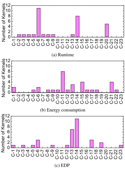
Figure 12: The number of kernels which benefit from each of the processor configurations listed in Table 7. These histogram diagrams show that the optimal processor configuration depends on the optimization goal.

CP Ub, are all considered asCP UL,1.4Ghz−CP Ub. The predictive

model for EDP was able to achieve a correct match for 30 of our 32 kernels, achieving a prediction accuracy of 93.6%.

For EDPInital,Accelerator and Host Config, andAccelerator

ConfigSVMsall achieve 100% accuracy. Only the finalSVM,Host

Config, is unable to achieve 100% accuracy, although, at this point in our model an incorrect prediction does not yield catastrophic results. Bothlud.k3andhisto.k3achieve their best performance when hosted by the big CPU, but both are predicted to be hosted by the little CPU. We speculate that this difficultly to accurately predict the host comes as a result of our compact set of features (due to the small number of training programs). However, these features are able to represent the intrinsic parts of each kernel, so are able to accurately predict the best device to execute each kernel. Beyond our featuretransfer_size, little information is given to theSVMto characterize how thehostprogram of each kernel will perform. Including more features, perhaps just to this final model, which are able to characterize how the host program performs is likely to solve this issue.

7.5 Optimal Processor Configurations

Figure 12 shows the number of kernels which perform best on each of the processor configurations we found useful in this work. Table 7 shows how eachConfig-Numcorresponds to a processor configuration, any configuration not included in this table never yielded an optimum result when optimizing any of our kernels for any of our metrics.

It can be observed that there is not a singular configuration which gives an optimum result over many kernels across performance, energy consumption and EDP. For example, C-20 (CP UB,2.0Ghz−

GP Ub) is an optimum configuration for 11 of our 32 kernels when

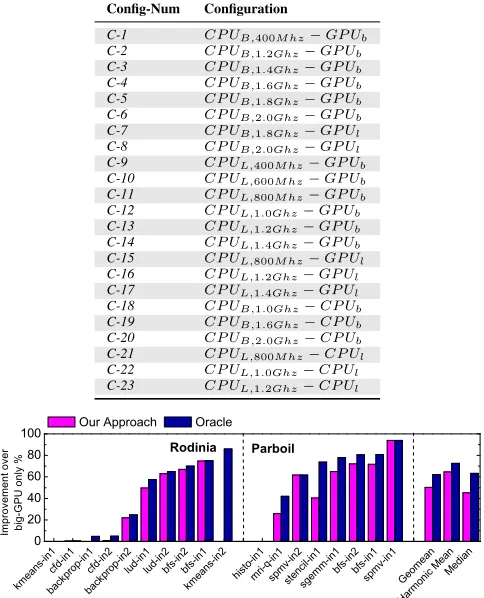
Table 7: Useful processor configurations in this work.

Config-Num Configuration

C-1 CP UB,400M hz−GP Ub

C-2 CP UB,1.2Ghz−GP Ub

C-3 CP UB,1.4Ghz−GP Ub

C-4 CP UB,1.6Ghz−GP Ub

C-5 CP UB,1.8Ghz−GP Ub

C-6 CP UB,2.0Ghz−GP Ub

C-7 CP UB,1.8Ghz−GP Ul

C-8 CP UB,2.0Ghz−GP Ul

C-9 CP UL,400M hz−GP Ub

C-10 CP UL,600M hz−GP Ub

C-11 CP UL,800M hz−GP Ub

C-12 CP UL,1.0Ghz−GP Ub

C-13 CP UL,1.2Ghz−GP Ub

C-14 CP UL,1.4Ghz−GP Ub

C-15 CP UL,800M hz−GP Ul

C-16 CP UL,1.2Ghz−GP Ul

C-17 CP UL,1.4Ghz−GP Ul

C-18 CP UB,1.0Ghz−CP Ub

C-19 CP UB,1.6Ghz−CP Ub

C-20 CP UB,2.0Ghz−CP Ub

C-21 CP UL,800M hz−CP Ul

C-22 CP UL,1.0Ghz−CP Ul

C-23 CP UL,1.2Ghz−CP Ul

kmea ns-in

1 cfd-in

1

back prop

-in1 cfd-in

2

back prop

-in2 lud-in

1 lud-in

2 bfs-in2bfs-in1

kmea ns-in

2

histo -in1

m ri-q-in1

spm v-in2 stenc

il-in1

sgem m-in

1 bfs-in2bfs-in1

spm v-in1

Geom ean

Harm onic

Mea n Med

ian 0

20 40 60 80 100

Im

p

ro

ve

m

e

n

t o

ve

r

b

ig

-G

P

U

o

n

ly

%

Our Approach Oracle

Rodinia Parboil

Figure 13: Optimization for EDP. Performance of our model com-pared to theOraclewhen different inputs are considered. Bench-marks names have either -in1 or -in2 appended to denote the differ-ent input sizes.

for energy consumption or EDP we would only achieve an optimum result for 4 and 3 kernels, respectively. Each configuration which performs well for one optimization goal does not perform well for the others. We can also see that the best number of kernels a configuration can optimize for at once is 11 (34%), and that there is a wide range of configurations which give optimizing performance for each metric. This shows the need for an approach that is able to spot the subtle differences in each kernel to optimize correctly.

7.6 Varying Input Sizes

Figure 13 shows how our model performs when we consider different inputs. Only some of the benchmarks provided us with methods to change their input. We have presented these results on a per-benchmark basis for EDP. However, the results per-kernel, and for each metric are very similar.

It can be observed that our approach performs well, even when optimizing the same benchmark with different inputs. In fact, for EDP, our model never gives a slowdown. Overall, we achieve 90% of theOracleperformance. Our approach is successful when input sizes differ as a benchmark’s input size will alter the execution of a kernel, thus, changing some features. Our model will treat this as anew, unseenkernel.

8.

Model Analysis

In this section we analyse the overall effectiveness of our model. First, we analyse the importance of each of our chosen features for each of our evaluation metrics. We then compare our model against other widely used machine learning classification techniques.

Figure 14: A Hinton diagram showing how each selected feature is likely to impact the performance for each model. Here, the larger the box, the more important a feature is.

Finally, we analyse the training and deployment overhead of using our approach.

8.1 Feature Importance

Figure 14 shows a Hinton diagram illustrating the importance of our features. The impact each feature has on each of our predictive models, for performance, energy consumption and EDP, can easily be seen. Here, the larger the box, the more significant a particular feature’s contribution to the prediction accuracy is. Along the x-axis is each feature, and along the y-axis is each metric, corresponding to each of our models. We calculate the importance of each metric though the information gain ratio.

It can be observed that comm-comp_ratio andtransfer_size

are important features when determining the correct processor configuration, independent of the optimizing metric. Each feature has a different level of importance for each metric, e.g.

transfer-work_ratiois extremely important when optimizing for Energy

Consumption, less important for runtime, and has little importance for EDP. This diagram shows the need for distinct models for different optimization goals.

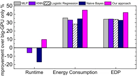
8.2 Alternative Predictive Modeling Techniques

Figure 15 shows the geometric mean of improvement of each kernel from the baseline achieved by our approach and four widely used classification techniques: Multi-layer Perceptron (MLP), K-Nearest Neighbours (KNN), Logistic Regression, and Naive Bayes. Each of the alternate predictive modeling techniques were trained and evaluated using the same methods and training data as our model.

Our approach outperforms each alternate technique for every optimization metric. None of the alternate techniques were able to achieve a positive geometric mean when optimizing for runtime, and were unable to yield better optimization results for any of the kernels or metrics we considered. This figure shows the success of our approach against alternate techniques. It is to note that the performance of these alternate modeling techniques may improve if there are more training examples to support the use of a richer set of features. However, we found that our hierarchicalSVMbased approach performs well on the available benchmarks.

8.3 Training and Deployment Overhead

R u n t i m e E n e r g y C o n s u m p t i o n E D P

- 2 0 - 1 0

0

1 0 2 0 3 0 4 0 5 0

Im

pr

ov

em

en

t o

ve

r b

ig

-G

PU

o

nl

y

% M L P K N N L o g i s t i c R e g r e s s i o n N a i v e B a y e s O u r a p p r o a c h

Figure 15: Comparisons to other predictive modeling techniques. Our hierarchical SVM based approach delivers the best overall performance.

9.

Conclusion

This paper has presented an automatic approach to map OPENCL tasks on heterogeneous mobile platforms, providing a significant performance improvement over comparative works. Central to our approach is a unified, machine learning based framework that predicts, for a given optimization criterion, which of the processors of the system to use to run the OPENCL program, and the clock frequency of the processor. The prediction is based on a set of code and runtime features of the program. Our model is built and trained off-line, and is fully automatic. We evaluate our approach on an ARM big.LITTLE mobile platform using a set of OPENCL benchmarks from the Rodina and the Parboil benchmark suites. Experimental results show that our approach consistently outperforms a comparative OPENCL mapping technique across three evaluation metrics: runtime, energy consumption and EDP. This translates to, on average, above 93% of the performance given by an ideal predictor.

Acknowledgement

The research was partly supported by the UK Engineering and Phys-ical Sciences Research Council (EPSRC) under grant agreements EP/M01567X/1 (SANDeRs) and EP/M015793/1 (DIVIDEND).

References

[1] H. Almatary et al. Reducing the implementation overheads of ipcp and dfp. InRTSS ’15.

[2] J. Ceng et al. Maps: an integrated framework for mpsoc application parallelization. InDAC ’08.

[3] P. Chakraborty et al. Opportunity for compute partitioning in pursuit of energy-efficient systems. InLCTES 2016.

[4] K. Chandramohan and M. F. O’Boyle. Partitioning data-parallel programs for heterogeneous mpsocs: time and energy design space exploration. InLCTES 2014.

[5] S. Che et al. Rodinia: A benchmark suite for heterogeneous computing. InIISWC ’09.

[6] G. Chen et al. Effisha: A software framework for enabling effficient preemptive scheduling of gpu. InPPoPP ’17.

[7] Y. Cho et al. Energy-reduction offloading technique for streaming media servers.Mobile Information Systems, 2016.

[8] C. Cummins et al. Synthesizing benchmarks for predictive modeling. InCGO 2017.

[9] K. Dev and S. Reda. Scheduling challenges and opportunities in integrated cpu+gpu processors. InESTIMedia’16.

[10] M. K. Emani et al. Smart, adaptive mapping of parallelism in the presence of external workload. InCGO, 2013.

[11] S. Eyerman and L. Eeckhout. Probabilistic job symbiosis modeling for smt processor scheduling. InASPLOS XV, 2010.

[12] E. Garzón et al. An approach to optimise the energy efficiency of iterative computation on integrated gpu–cpu systems.The Journal of Supercomputing, 2016.

[13] D. Grewe et al. Portable mapping of data parallel programs to opencl for heterogeneous systems. InCGO ’13.

[14] D. Grewe et al. A workload-aware mapping approach for data-parallel programs. InHiPCA, 2011.

[15] D. Grewe et al. Opencl task partitioning in the presence of gpu contention. InLCPC, 2013.

[16] N. Guan et al. Schedulability analysis of preemptive and nonpreemptive edf on partial runtime-reconfigurable fpgas.ACM TODAES, 2008. [17] C. Imes and H. Hoffmann. Bard: A unified framework for managing

soft timing and power constraints. InSAMOS, 2016.

[18] Jääskeläinen et al. Pocl: A performance-portable opencl implementa-tion.Int. J. Parallel Program., 2015.

[19] W. Jia et al. Gpu performance and power tuning using regression trees. ACM Trans. Archit. Code Optim., 2015.

[20] R. Kaleem et al. Adaptive heterogeneous scheduling for integrated gpus. InPACT ’14.

[21] S. S. Latifi Oskouei et al. Cnndroid: Gpu-accelerated execution of trained deep convolutional neural networks on android. InMM ’16, 2016.

[22] J. Lee, M. Samadi, and S. Mahlke. Orchestrating multiple data-parallel kernels on multiple devices. InPACT ’15, .

[23] M. S. Lee et al. Accelerating bootstrapping in fhew using gpus. In ASAP ’15, .

[24] J. Leng et al. Gpuwattch: enabling energy optimizations in gpgpus. In ISCA 2013.

[25] K. Ma et al. Greengpu: A holistic approach to energy efficiency in gpu-cpu heterogeneous architectures. InICPP 2014.

[26] A. Magni et al. Automatic optimization of thread-coarsening for graphics processors. InPACT ’14.

[27] D. Majeti et al. Automatic data layout generation and kernel mapping for cpu+gpu architectures. InCC 2016.

[28] P.-J. Micolet et al. A machine learning approach to mapping streaming workloads to dynamic multicore processors. InLCTES 2016. [29] W. Ogilvie et al. Minimizing the cost of iterative compilation with

active learning. InCGO, 2017.

[30] P. Pandit and R. Govindarajan. Fluidic kernels: Cooperative execution of opencl programs on multiple heterogeneous devices. InCGO ’14. [31] H. Park et al. Zero and data reuse-aware fast convolution for deep

neural networks on gpu. InCODES+ISSS 2016.

[32] J. Ren et al. Optimise web browsing on heterogeneous mobile

platforms: a machine learning based approach.

[33] J. Ren et al. Optimise web browsing on heterogeneous mobile

platforms: a machine learning based approach. InINFOCOM, 2017. [34] A. K. Singh, M. Shafique, A. Kumar, and J. Henkel. Mapping on

multi/many-core systems: Survey of current and emerging trends. In DAC 2013.

[35] A. Snavely and D. M. Tullsen. Symbiotic jobscheduling for a simulta-neous multithreaded processor. InASPLOS IX, 2000.

[36] J. A. Stratton and others. Parboil: A revised benchmark suite for scientfic and commercial throughput computing.

[37] G. Tournavitis et al. Towards a holistic approach to auto-parallelization: integrating profile-driven parallelism detection and machine-learning based mapping. InPLDI ’09.

[38] S. Verdoolaege et al. Polyhedral parallel code generation for cuda. ACM TACO, 2013.

[39] Z. Wang and M. O’Boyle. Mapping parallelism to multi-cores: a machine learning based approach. InPPoPP ’09.

[40] Z. Wang and M. F. O’Boyle. Partitioning streaming parallelism for multi-cores: a machine learning based approach. InPACT, 2010. [41] Z. Wang et al. Integrating profile-driven parallelism detection and

machine-learning-based mapping.ACM TACO, 2014.

[42] Z. Wang et al. Automatic and portable mapping of data parallel programs to opencl for gpu-based heterogeneous systems.ACM TACO, 2015.