warwick.ac.uk/lib-publications
Manuscript version: Author’s Accepted Manuscript
The version presented in WRAP is the author’s accepted manuscript and may differ from the
published version or Version of Record.
Persistent WRAP URL:
http://wrap.warwick.ac.uk/116197
How to cite:
Please refer to published version for the most recent bibliographic citation information.
If a published version is known of, the repository item page linked to above, will contain
details on accessing it.
Copyright and reuse:
The Warwick Research Archive Portal (WRAP) makes this work by researchers of the
University of Warwick available open access under the following conditions.
© 2019 Elsevier. Licensed under the Creative Commons
Attribution-NonCommercial-NoDerivatives 4.0 International http://creativecommons.org/licenses/by-nc-nd/4.0/.
Publisher’s statement:
Please refer to the repository item page, publisher’s statement section, for further
information.
General Job Lengths Under the SQ(
d
) Policy
ABSTRACT
In this paper, we study the mean-field behavior of large-scale sys-tems that consist ofN(large) identical parallel processor sharing servers with Poisson arrival process having intensityN λand gen-erally distributed job lengths under the randomized SQ(d) load balancing policy. Under this policy, an arrival is routed to the server with the least number of progressing jobs amongdrandomly chosen servers. The limit of the empirical distribution is then used to study the statistical properties of the system. In particular, this shows that in the limit asNgrows, individual servers are statistically in-dependent of others (propagation of chaos) and more importantly, the equilibrium point of the mean-field is insensitive to the job length distributions that has important engineering relevance for the robustness of such routing policies used in web server farms. We use a framework of measure-valued processes and martingale techniques to obtain our results. We also provide numerical results to support our analysis.
CCS CONCEPTS
•Networks→Network performance analysis;
KEYWORDS
Mean-field limit, Fixed-point, Insensitivity, Measure-valued pro-cesses
ACM Reference Format:
. 2018. The Mean-field Behavior of Processor Sharing Systems with General
Job Lengths Under the SQ(d) Policy. InProceedings of ACM PERFORMANCE
conference (IFIP PERFORMANCE 2018).ACM, New York, NY, USA, Article 4,
25 pages. https://doi.org/10.1145/nnnnnnn.nnnnnnn
1
INTRODUCTION
The emergence of the cloud computing paradigm and other central-ized applications result in server farms that contain large numbers of servers to process the incoming job requests. The front end job dispatchers route an arriving job to one of the servers that pro-vide minimal response times as the tasks in most cases are delay sensitive[20]. Therefore the key challenge in these systems is to design low complex load balancing algorithms that results in effi-cient use of resources thereby good system performance. In server farms, the resources are shared by processing requests in a round-robbin manner with small time granularity. This model can be well approximated by the processor sharing model [17, 36] where the
Permission to make digital or hard copies of part or all of this work for personal or classroom use is granted without fee provided that copies are not made or distributed for profit or commercial advantage and that copies bear this notice and the full citation on the first page. Copyrights for third-party components of this work must be honored. For all other uses, contact the owner /author(s).
IFIP PERFORMANCE 2018, December 2018, Toulouse, France © 2018 Copyright held by the owner/author(s). ACM ISBN 978-x-xxxx-xxxx-x/YY/MM. . . $15.00 https://doi.org/10.1145/nnnnnnn.nnnnnnn
processing speed of a server is equally shared by all the progressing jobs.
In practice, the server farms such as Cisco Local Director, IBM Network Dispatcher, Microsoft Sharepoint use the classical Join-the-shortest-queue ( JSQ) policy to achieve the load balancing. It was shown in [14, 34] that the JSQ policy is nearly optimal and further, it is robust to the job length distributions since it is nearly insensitive. The notion of insensitivity implies that the stationary distribution of occupancy depends only on the mean job lengths but not on the type of job-length distributions. For large scale systems that contain hundreds of thousands of servers, the JSQ policy requires the information about the number of progressing jobs at all the servers. However it was shown in [6, 21–24, 32] that a randomized routing scheme SQ(d) based on sending jobs to the best amongst
drandomly chosen servers can achieve almost the same gains at a much smaller sampling cost. This policy achieves near optimal performance even ford=2 and hence, led to the popularization of the so-calledpower-of-2terminology.
In [32], under the assumption of exponential service time distri-butions, the SQ(d) policy withd=2 was introduced for multi-server systems havingN severs with FCFS service discipline and the job arrival process is a Poisson process with rateN λ, where the policy of routing the smaller of two randomly sampled servers was studied. Since under the SQ(d) or power-of-drouting policy, the servers are coupled in a finiteNsystem, the exact analysis of the system is not tractable and it is extremely difficult. Their key contribution was that by first taking the limit asN→ ∞the system decouples into independent queues where the limiting empirical distribution of a queue is described by a deterministic non-linear equation called the mean-field or hydrodynamic limit. The property of decoupling between servers asN → ∞is called propagation of chaos. More-over they showed that the limit of the stationary distribution of the queues corresponds to the equilibrium or fixed point of the mean field equations (MFE) and the proof relies on the fact that the mean-field has quasi-monotonicity property. Furthermore, the fixed point of the MFE that represents the stationary distribution of a queue shows a dramatic reduction in the average response time due to the fact that the occupancy (Q) has tail distribution satisfying a super-exponential decay given by Pr(Q≥k)=(λµ)2
k−1
instead of(λµ)kthat would be the case if uniform routing had been used. Later the analysis is extended to the SQ(d) policy withd>2 in [21] where it was shown that the fixed point of the MFE
satis-fies Pr(Q≥k)=(λµ)
dk−1
d−1. These nice conclusions reflect that the mean-field techniques can help us to obtain deeper insights about a large-scale complex stochastic system when the exact analysis is not tractable.
been recently addressed with some partial progress and simulation observations that we recall later in this section. This is because for queuing systems with general service times, the job occupancy process (Queue-length process) is not Markov and this limits us in extending the analysis directly from exponential case to the gen-eral distributions case. In that case one needs to Markovianize the system by considering the occupancy state as well as the age or residual service times of the jobs in service which makes the mean-field analysis a challenging task. However, it is very important to make progress on understanding the large-scale multi-server system behavior when we employ the SQ(d) policy since more real-istic models need us to dispense with the exponential job length hypothesis. For example, the service time distributions are Log-normal in call centers [8], and Gamma distributed in automatic teller machines (ATMs) [18] etc. Therefore it is necessary to study the impact of SQ(d) routing scheme when job lengths are generally distributed.
In this paper we consider a multi-server large scale processor sharing system with the generally distributed job lengths with finite mean 1µ under the SQ(d) policy. Earlier, the case with groups of heterogeneous servers under the assumption of exponential job lengths was studied in [22, 23] using mean-field techniques. In particular, they established the global asymptotic stability (GAS) of the mean-field limit that also establishes that the fixed point of the MFE corresponds to the limiting stationary distribution of a server occupancy.
The focus in this paper is to understand the probabilistic behavior of systems with a large number of servers by studying the limiting behavior when the number of servers goes to infinity. We show that in this context the limit of the empirical distribution satisfies a deterministic equation called the mean-field or hydrodynamic limit. One of the key insights we seek is how the distribution of the job lengths affects the mean-field behavior. We show that as
N→ ∞any finite set of servers become statistically independent and moreover the fixed point of the mean field only depends on the mean job lengths and not their distributions, the property termed as insensitivity. It is well known that Processor Sharing systems are insensitive to the service time distributions in equilibrium for Poisson inputs, and thus our result shows that this property is inherited under randomized SQ(d) routing. In prior works [6, 23] evidence of this property was presented via simulations but without complete proof.
We now discuss some of the results on the large-scale multi-server systems with general job length distributions under the SQ(d) policy. The SQ(d)policy for processor sharing, FIFO, and LIFO with preemptive resume models with general job length dis-tributions in the homogeneous context were studied in [6] under theansatzhypothesis that the underlying stationary distribution of the occupancy of the Markov process converges to a unique limiting distribution and any finite set of servers are asymptotically independent using the cavity method. As we show in Section 5.2, theansatzcarries the necessary and sufficient conditions needed to conclude insensitivity for processor sharing systems. This is because each individual server must have state dependent Poisson arrivals which is a consequence of the assumption of asymptotic independence of servers or propagation of chaos and furthermore,
existence of unique stationary distribution is essential to conclude insensitivity. Bramson [7] succeeded in proving theansatzonly for the case of FIFO models with job length distributions having decreasing hazard rate functions.
Recently the FIFO case with generally distributed service times has been revisited in [1] via a mean-field approach where they show that the joint process that counts the jobs at a server and the age of the job in service has a mean-field that is described by a set of PDEs. However the analysis is only restricted to the finite time or transient case and no results are given for the stationary regime. They also established the propagation of chaos for the individual queues for any finite timetin the limiting system. However, in the processor sharing case, the analysis is now more complicated because in addition to the occupancy process one needs to keep track of the ages of all the jobs in the system. This results in a Markov process onÐn∈Z
+(n,ℜn+)and the analysis and proofs are much more difficult because the ages do not increase linearly at the rate of processing speed of the server but the rate depends on the server occupancy or the first coordinate of the Markov process. This requires us to consider a measure-valued Markov process representation.
The use of measure-valued processes to deal with general service time distributions is natural. In [13] it was used to study the fluid limit of a singleGI/GI/1 processor sharing system in critically loaded regime. The steady state analysis of the fluid limit established in [13] is considered in [25]. However, the mean-field limit that we study in this paper has not been addressed for processor sharing systems under SQ(d). The analysis is now more difficult because the mean-field limit represents the dynamics of a non-linear Markov process and the arrival rate to each server in the limiting system takes a specific form under the SQ(d) policy.
Recently there has been interest in P ULL based policies such as Join-Idle-Queue ( JIQ)[20]. In JIQ the dispatcher stores the identities of servers that are idle in a memory and an arrival is routed to a ran-domly selected idle server if there are any available in the list at the dispatcher, otherwise the job is routed to a server chosen uniformly at random. In [29], it was shown that under sub-critical system load, the steady state probability of waiting vanishes asN → ∞. However, under high load, since random routing is used, there are often no idle servers in the list and it is observed in [20, 33] that the SQ(d) performs better than JIQ. To overcome this, extensions to JIQ have been considered. In one approach, the dispatcher stores the identities of all the servers with number of progressing jobs less than or equal to some threshold value such as one[20]. An arrival is routed to a randomly selected server from the list at the dispatcher if there are any available, otherwise the job is routed to a server chosen uniformly at random. In the second approach, the JIQ is combined with the SQ(d) where when there are no idle servers, the destination server is chosen according to the SQ(d) policy[33]. These extensions increase complexity significantly. Therefore un-derstanding the impact of the SQ(d) policy when job lengths are general is an important problem.
Main contributions:The main contributions of this paper are listed below:
in each possible server state converges in distribution to a unique deterministic measure-valued process called as the mean-field limit. As a consequence of this, we also establish the propagation of chaos for any finite timet.
•Insensitivity of Equilibrium point of the MFE:We then show that the partial differential equation (PDE) that describe the mean-field limit has a unique equilibrium point. Further-more, the equilibrium point is insensitive to the job length distributions. We also provide simulation results that support the insensitivity and the GAS of the equilibrium point. This result has significant engineering implications in practice since the load balancing for large-scale processor sharing systems appear in server farms.
Organization of the paper
The rest of the paper is organized as follows: In Section 2, we intro-duce the system model, the SQ(d)policy, notation, and a Markovian description of the system by using a state descriptor. In Section 3, we give the main results of this paper. We then study the unique-ness of the fixed-point of the mean-field limit and its insensitivity in Section 4. After that, in Section 5, we provide a discussion on the relationship between propagation of chaos in the stationary regime and the mean-field where we also recollect existing works regarding this. In Section 5, we also provide numerical results that support insensitivity and GAS of the fixed-point of the mean-field limit. Finally, we conclude in Section 6 with a discussion on future work. The proofs are provided in Appendix (Section 7).
2
SYSTEM MODEL AND PRELIMINARIES
We first introduce the system model and the routing policy consid-ered in this paper.
We consider a large-scale system that containsN identical pro-cessor sharing servers each having unit processing rate. Therefore if there arenjobs in progress at a server, then each job is processed at the rate of 1
n.
Jobs arrive into the system according to a Poisson process with rateN λand there is a central job dispatcher that routes an incoming job to one of the servers according to the SQ(d) routing policy described below.
Definition1. The SQ(d)Routing:
An incoming job is routed to the server with least number of ongoing jobs amongdchosen servers uniformly at random with replacement1 . The ties if there are any, are broken by choosing a server uniformly at random. Thedrandomly chosen servers are called as potential destination servers and the server that is picked from the potential destination servers to route the arrived job is called as the destination server.
We assume that the job lengths have general cumulative distribu-tion funcdistribu-tionG(·)with density functionд(·)such that the average job length is equal to1µ. The hazard rate function of the job length
1
Although we consider that servers are picked with replacement for simplification of the analysis, in both the cases with or without replacement, asN → ∞, they would result in the same mean-field limit. For largeNsystems, simulation results also support this.
distribution is denoted byβ(·)= д(·)
G(·)
. For the system to be in stable
region, we must haveλ<µ.
Notation:We now introduce the mathematical notations that we use in rest of the paper. LetZ,Rdenote the space of integers and real numbers, respectively. The space of non-negative integers and non-negative real numbers are denoted byZ+,R+, respectively.
For any given metric spaceE, letKb(E),Cb(E),Ck(E) be the space of real-valued bounded measurable, bounded continuous, and continuous functions with compact support, respectively. Further, letC1(E)be the space of once continuously differentiable functions defined onE. The subset of functions inC1(E)that are bounded functions whose first derivatives are also bounded is denoted by
C1
b(E)and the space of functions with compact support inC1(E)is denoted byC1
k(E). For any functionf ∈ Kb(E), we define
∥f∥=sup
x∈E
|f(x)|. (1)
The spaceCb(E)is equipped with the uniform topology,i.e., a sequence of functions{fn}n≥1inCb(E)is said to converge to a
functionf ∈ Cb(E)if∥fn−f∥ →0 asn→ ∞. We next define for any functionf ∈ C1
b(E),
∥f∥1=∥f∥+∥f
′∥,
(2)
wheref′is the first derivative off. The spaceC1
b(E)is equipped with the topology induced by the norm∥·∥1. For a functionf ∈
C1
b(Rn+), we define a functionfÍ′ :R+n7→ Ras follows
f′
Í(x1,· · ·,xn)=
1
n
n
Õ
i=1
∂f(x1,· · ·,xn)
∂xi .
(3)
For given metric spaceE, let the Borelσ-algebra be denoted by
B(E). The space of finite non-negative measures defined onEis represented byMF(E)and the space of probability measures is denoted byM1(E). For a Borel setB∈ B(E), the measure value of the setBwith respect to the measureνis given byν(B)and the measure value at an elementy∈Eis given byν({y}). Further, the Dirac measure with unit mass atx ∈Eis denoted byδx. We also define a set of probability measuresMN
1 (E)as follows
M1N(E)={ν∈ M1(E):Nν(B) ∈ Z+,∀B∈ B(E)}. (4)
We next define for anyϕ∈ Cb(E),ν ∈ MF(E),
⟨ν,ϕ⟩=
∫
y∈E
ϕ(y)dν(y). (5)
The spaceMF(E)is equipped with the weak topology,i.e., a se-quence{νn}inMF(E)is said to converge weakly toν ∈ MF(E)if and only if⟨νn,ϕ⟩ → ⟨ν,ϕ⟩asn→ ∞for allϕ∈ Cb(E). We recall that ifEis a Polish space, thenMF(E)equipped with the weak topology is also a Polish space.
We next introduce the notations that are required to model a processor sharing system evolution. To model the system evolution by a Markov process, we consider that the state of a server is given by(n,a1,· · ·,an)whereaiindicates the age of thei
th
progressing job at timetthat entered the server at timeTi (t ≥Ti) is given by
ai=
∫ t
s=Ti
1
γ(s)ds. (6)
LetUnbe the set of all possible states of a server when there aren progressing jobs,i.e.,
Un={(n,a1,· · ·,an):ai ∈ R+,1≤i≤n}. (7)
When there are no progressing jobs, then the server state lies in the set
U0={0}. (8)
Therefore at any given timet, the state of a server lies in the set
U =∪n∈Z+Un. (9)
Without loss of generality, we indicate an element(n,u1,· · ·,un) ∈
Uforn≥0 byu. Foru=(n,u1,· · ·,un)andv=(m,v1,· · ·,vm),
we define the metric
dU(u,v)=
( Ín
i=1|ui −vi| ifn=m
∞ otherwise.
(10)
We say that a sequence{u
n,n ≥1}inU converges tou ∈U if limn→∞dU(un,u)=0.
For any Borel setB∈ B(U), we define the indicator function of
Bas
I{B}(u)=
(
1 ifu∈B 0 otherwise.
(11)
Further, we define a function1:U 7→ Ras
1(u)=1, (12)
foru∈U.
Any measureν ∈ MF(U)restricted to the spaceU0is a Dirac
measure with mass at(0). Further, forn≥1, we say that the measure
ν∈ MF(U)is absolutely continuous atx∈Unifν({x})=0 and the measureνis called absolutely continuous with respect to Lebesgue measure ifν({y})=0 for ally∈Un,n≥1. We say that a function
f :U7→ Ris differentiable if for everyi≥1, ∂f(i,x1,···,xi)
∂xj exists
for every 1≤j ≤iat every(x1,· · ·,xi) ∈ Ri+. Hence a function
of the typef =I{U
n}, forn ≥ 1, that we use frequently in our analysis is differentiable.
We next define the following two functions that are used in Assumption 2 in order to establish the mean-field limit. The first function isΞ:U 7→ Rdefined as
Ξ(n,x1,· · ·,xn)=n, (13)
for(n,x1,· · ·,xn) ∈U. The second function,ϒ:U7→ Ris defined
as
ϒ(n,x1,· · ·,xn)= (
0 forn=0,
x1+· · ·+xn otherwise.
(14)
We next define the transition operators on functions and mea-sures that we use in describing the time evolution of the system. For anyu∈Un,n≥1 and forb>0, if a sever lies in stateu∈Un at timet, then if there are no arrivals or departures at this server in the interval(t,t+b], then its updated state at timet+bis denoted by
τb+(n,u1, . . . ,un)=
n,u1+
b n,u2+
b
n,· · ·,un+ b n
(15)
and
τb+(0)=(0). (16)
Further, for anyy>0,f ∈ Kb(U), we define a mapping
τy :Kb(U) → Kb(U) (17)
satisfying
τyf(u)=f(τy+u). (18)
Fory>0, now let us define a shifted measureτyν ∈ MF(U)such that for any Borel setB ∈ B(U), we have
τyν(B)=ν(τy+(B)). (19)
Forν∈ MF(U), the measureτyν∈ MF(U)satisfies
⟨τyν,f⟩=⟨ν,τyf⟩ (20)
for allf ∈ Kb(U). The Riesz-Markov-Kakutani theorem [27, 30] implies the existence of the unique measureτyνsatisfying equa-tion (20). For the measure-valued Markov process (νNt ,t ≥ 0) that describes the system evolution, equation (20) plays crucial rule in computing the expression of the generator of the process
(νNt ,t≥0). In particular, by using equation (20), the information about change in the process(νNt ,t ≥0)in a given time interval can be treated as a change in the functionf. Based on this idea, by choosing the class of functions of the typeνNt 7→ ⟨νtN,ϕ⟩for
ϕ ∈ C1
b(U), one can compute the expression of the generator of the Markov process(νtN,t ≥0).
We next define a norm on the measureν∈ MF(U)that we use in proving the uniqueness of a solution to the MFE given an initial point. Forν∈ MF(U),⟨ν,ϕ⟩is a continuous linear operator on the space of functionsϕ∈ Cb(U), we define
∥ν∥= sup
ϕ∈ Cb(U) |⟨ν,ϕ⟩|
∥ϕ∥ . (21)
WhenHis a Polish space, letDH([0,T]),DH([0,∞))denote the càdlàg2functions that take values inHdefined on[0,T],[0,∞), respectively. The space of the continuous functions that take values inHdefined on[0,T],[0,∞)are denoted byCH([0,T]),CH([0,∞)), respectively. We assume that the spacesDH([0,T]),DH([0,∞))are equipped with the SkorokhodJ1-topology and in that case, they are
Polish spaces. For two local martingales(Mt1,t≥0)and(M2t,t ≥0), we denote the covariation and quadratic variation inDR([0,T])by
(<M1
·,M
2
· >t,t ≥0)and(<M1· >t,t ≥0)=(<M1·,M1· >t,t ≥ 0), respectively.
In this paper, we work withH −valued stochastic processes whereH=MF(U). We assume that the considered stochastic pro-cesses are random elements defined on(Ω,F,P)with sample paths lying inDH([0,∞)). The spaceDH([0,∞))is equipped with the Borelσ−algebra generated by the open sets under the Skorokhod
J1−topology [4]. A sequence{Xn}ofH-valued càdlàg processes
defined on(Ωn,Fn,Pn)is said to converge in distribution to aH -valued càdlàg processX defined on(Ω,F,P)if, for every bounded, continuous, real valued functionalF:DH:[0,∞) → R, we have
lim
n→∞En(F(Xn))=E(F(X)) (22)
2
where the expectation operatorsEn,Eare defined with respect to
Pn,P, respectively. The convergence of{Xn}in distribution toX is denoted byXn⇒X. Law of a random variableXis denoted by
L(X).
Markovian description: We first introduce the system state descriptor that represents the system state at any given timet. We then describe the system evolution.
In our analysis, we consider age of each progressing job in mod-eling the system by a Markov process. At any timet, a server’s state is represented by(n,a1,· · ·,an)wherendenotes the number
of progressing jobs at the server at timetandai denotes the age of theithprogressing job at timet. If a server has no job at time
t, then its state is considered to be(0). We now define the system state descriptor as follows.
Definition2. System State Descriptor
If the state of server“i”at timetis denoted bysit=(ni,a1,i,a2,i,· · ·,an
i,i),
then the system state at timetis defined by the measure valued process
νtN =
N
Õ
i=1
δ(si
t) (23)
whereδ(n,x1,···,xn)denotes the Dirac measure with unit mass at
(n,x1,· · ·,xn). Note thatνtN({(m,z1,· · ·,zm)})denotes the number of servers with state(m,z1,· · ·,zm)at timet.
Once we define the state descriptor, the time evolution of the sys-tem is modeled by tracking the time evolution of the the measure-valued process(νtN,t ≥ 0). For givenh > 0 andνtN, to know the value ofνN
t+h, we need to exactly track how each server state changes in the time interval(t,t+h]. In this interval, there can be no event (arrival or departure) or some events(arrivals and de-partures) can occur in the system. The departure events can be modeled by using hazard rate functionβ(x) = д(x)
G(x)
that defines
the instantaneous rate of departure of a job conditioned on its age value equal tox. Precisely, if a job achieves agex at timet, then it departs in the interval(t,t+y]with probability given by
G(x+y)−G(x)
G(x) =β(x)y+o(y). When the number of progressing jobs
does not change at a server with state say(n,a1,· · ·,an)at timet
in the interval(t,t+h], then its state becomesτ+
h(n,a1,· · ·,an)at
timet+h. By assuminghis a small value, we consider that multiple events do not occur in the interval(t,t+h].
3
MAIN RESULTS
We now present the main results of this paper.
The goal of this paper is to study the limit of the following normalized process(νtN,t≥0)defined as
νtN =νNtN (24)
whenN → ∞. Furthermore, we would like to study the fixed-point of the limit to obtain some Engineering insights.
We next state the following simple result on probability of choos-ing a server with state(n,l1,· · ·,ln)as the destination server upon
an arrival.
Lemma1. SupposeνtN =η, then according to the SQ(d)routing
policy, if a job arrives at timet, the probability that it is routed to a server with state(n,l1,· · ·,ln)is equal to
pr(n,l1,· · ·,ln;η)=
η{(n,l1,· · ·,ln)}
N Φn
η
N
, (25)
where
Φn
η
N
=(Rn(
η
N)d−Rn+1( η N)d)
(Rn(Nη) −Rn+1( η N))
(26)
andRn(Nη)=
Í∞
j=nη({Uj})
N represents the fraction of servers with at leastnjobs at timet.
The proof of Lemma 1 is given in Appendix 7.1.
Our analysis shows that under the SQ(d) policy, the probability of choosing a server as destination server given by (25) has the following implications in the limiting system asN → ∞. Once we establish the mean-field(νt,t≥0), in the limiting system, due to propagation of chaos, each individual server has Poisson arrival process having rateλΦn(νt)when there arenprogressing jobs at timet.
Before stating our results precisely, we briefly summarize our analysis and findings below.
Sketch of the analysis:In this paper, we show the weak convergence of the measure-valued Markov process(νNt ,t ≥0)to the mean-field
limit via the following arguments. We first construct the Dynkin martingale[11] in Theorem 1 associated with the process(νtN,t ≥
0). We then state the result on establishing the mean-field limit in
Theorem 2. In the first part of Theorem 2, we show that there exists unique solution to the MFE for given initial point. In the second part of Theorem 2, we show that the process(νNt ,t ≥0)converges to the
unique solution of the MFE referred as the mean-field solution. For this, we use the constructed martingale Theorem 1 to establish the tightness of the process(νNt ,t ≥0)by using Jakubowski’s criteria[10]. After
that, by showing that the sequence of martingales converge to the null process asN → ∞and the tightness of(νNt ,t≥0), we get that every
limit point satisfies the MFE. Further, since there exists unique mean-field solution for given initial point, under the assumption ofνN0 ⇒ν0 whereν0is a deterministic measure inM1(U), we get that all the limit points have identical distribution coinciding with that of the unique deterministic field solution. This establishes the mean-field limit and as a consequence, we also establish the propagation of chaos for any finite timetin Theorem 4. In order to study the fixed-point of the mean-field, we translate the integral form of the MFE to the PDEs satisfied by the mean-field. Finally, we state our main result on the insensitivity of the fixed-point of the mean-field in Theorem 3. We also provide some insights about the stationary behavior of the limiting system in Section 5 where we also discuss drawbacks of [6] in concluding the insensitivity.
The starting point of our analysis depends on finding a suitable martingale process that can be used to establish the mean-field limit. For this, the starting step is to characterize the Markov pro-cess(νtN,t ≥0)and finding its generatorAN(·). We consider the filtration defined by
FtN =σ(νsN(B):s≤t,B∈ B(U)). (27)
Theorem1. The process(νtN,t ≥0)is a Feller-Dynkin process[10,
11] ofDMF(U)([0,∞)). Letϕ∈ C1
0)defined as
MtN(ϕ)=⟨νtN,ϕ⟩ − ⟨ν0N,ϕ⟩ −
∫ t
s=0
AN⟨νsN,ϕ⟩ds (28)
is a square integrableFtN-martingale and it is right continuous with left limits (RCLL) process. Further, forϕ,ψ ∈ C1
b(U), the mutual variation of(MtN(ϕ),t≥0)with(MtN(ψ),t ≥0)is given by
<MN(ϕ)·,MN· (ψ)>t=
∫ t
s=0
∞
Õ
n=1 n
Õ
j=1 ∫
x1
· · ·
∫
xn
β(xj)
n
× (ϕ(n−1,x1,· · ·,xj−1,xj−1,xj+1,· · ·,xn) −ϕ(n,x1,· · ·,xn))
× (ψ(n−1,x1,· · ·,xj−1,xj−1,xj+1,· · ·,xn) −ψ(n,x1,· · ·,xn))
×dνsN(n,x1,· · ·,xn)
+N λhνsN({0}) N Φ0
νN s
N
!
(ϕ(1,0) −ϕ(0))(ψ(1,0) −ψ(0))
+
∞
Õ
n=1 n+1 Õ
j=1 ∫
x1
· · ·
∫
xn
1
N(n+1)Φn
νN s
N
!
× (ϕ(n+1,x1,· · ·,xj−1,0,xj,· · ·,xn) −ϕ(n,x1,· · ·,xn))
× (ψ(n+1,x1,· · ·,xj−1,0,xj,· · ·,xn) −ψ(n,x1,· · ·,xn))
×dνsN(n,x1,· · ·,xn) i
!
ds. (29)
.
The proof of Theorem 1 is given in Appendix 7.2.
We now look at establishing the mean-field limit. For this, we require the following assumptions:
Assumption 1. The hazard rate functionβ(·)satisfies
β∈ Cb(R+)and∥β∥<∞. (30)
Assumption 2. The sequence of initial measures of the normal-ized measure-valued processes(νtN,t ≥0)satisfy
(νN0,⟨νN0 ,Ξ⟩,⟨νN0,ϒ⟩) ⇒ (ν0,⟨ν0,Ξ⟩,⟨ν0,ϒ⟩) (31)
whereν0 ∈ M1(U) is absolutely continuous measure satisfying
⟨ν0,Ξ⟩<∞and⟨ν0,ϒ⟩<∞.
Definition3. Mean-field equations (MFE): The following
evo-lution equations are referred to as the MFE with initial pointη0 ∈
M1(U)satisfied by a process(ηt ∈ M1(U),t ≥0) ∈ CM1(U)([
0,∞)),
for allϕ∈ Cb(U),
⟨ηt,ϕ⟩=⟨η0,τtϕ⟩+ ∫ t
r=0
∞
Õ
n=1 n
Õ
j=1 ∫
x1
· · ·
∫
xn
β(xj) n
× τt−rϕ(n−1,x1,· · ·,xj−1,xj+1,· · ·,xn) −τt−rϕ(n,x1,· · ·,xn)
×dηr(n,x1,· · ·,xn)
+λ
ηr({0})Φ0 ηr(τt−rϕ(1,0) −τt−rϕ(0))
+
∞
Õ
n=1 n+1 Õ
j=1 ∫
x1
· · ·
∫
xn
1
(n+1)Φn ηr
× (τt−rϕ(n+1,x1,· · ·,xj−1,0,xj,· · ·,xn) −τt−rϕ(n,x1,· · ·,xn)),
×dηr(n,x1,· · ·,xn) !
dr, (32)
whereΦn ηr=(Rn(ηr)
d−R n+1(ηr)d)
(Rn(ηr)−Rn+1(ηr))
andRj(ηr)=Í∞
n=jηr(Un).
Any solution of the above equation is referred to as the mean-field solution. Note that since forϕ ∈ Cb(U),t 7→ ⟨ηt,ϕ⟩is a continuous mapping andCb(U)is a separating class ofM1(U),
t 7→ηtis continuous and hence any mean-field solution belongs to the setCM
1(U)([
0,∞)).
We next state our main result of the paper.
Theorem2. We establish the following two results
• There exists unique solution inCM
1(U)([
0,∞))satisfying the
MFE for given initial pointν0 ∈ M1(U). Furthermore, if
(ν1
t,t ≥0)and(ν2t,t ≥0)are two mean-field solutions that
start at the initial measuresν1
0 ∈ M1(U),ν 2
0 ∈ M1(U), re-spectively, then
∥ν1 t−ν2
t∥ ≤ ∥ν10−ν 2 0∥e
(2∥β∥+8d2λ)t.
(33)
• If the sequence{ν0N}satisfies the assumption 2, we then have for everyT >0,(νNt ,0≤t≤T) ⇒ (νt,0≤t ≤T)where the
process(νt,0≤t ≤T)is a deterministic process referred to
as the mean-field limit is the unique solution of the MFE(32)
with initial pointν0.
The proof of above Theorem 2 is given in Appendix 7.3. We now look at the probabilistic interpretation to the MFE. By using the propagation of chaos result that we state later in this sec-tion,νtrepresents the distribution of a server state in the limiting system. We next obtain the partial differential equations satisfied by the mean-field limit by using MFE (32). Sinceν0is absolutely
con-tinuousw.r.t.Lebesgue measure, then at everyt ≥0,νtis also ab-solutely continuous resulted from the fact thatν0is absolutely
con-tinuous and the mappingt7→νtis continuous. Letpt(0)denotes
νt({0})andpt(n,x1,· · ·,xn)denotes the Radon-Nikodym
deriva-tive of the measureνtw.r.t.Lebesgue measure at(n,x1,· · ·,xn). Let us define the processPt =(Pt(u),u∈U)as
Pt(n,y1,· · ·,yn)= ∫ y1
x1=0
· · ·
∫ yn
xn=0
pt(n,x1,· · ·,xn)dx1· · ·dxn.
(34) HencePt(n,y1,· · ·,yn)denotes the probability that a server hasn
jobs andithjob, 1≤i≤n, has age atmostyi in the limiting system at timet.
Corollary1. The processPt=(Pt(u),u∈U)satisfies the PDEs
dPt(0)
dt =
∫ ∞
y=0
β(y)
∂P
t(1,y)
∂y
dy−λΦ0(Pt)Pt(0), (35)
forn≥1,
dPt(n,y1,· · ·,yn)
dt =−
n
Õ
i=1
1
n
∂Pt(n,y1,· · ·,yn) ∂yi
+
n+1 Õ
j=1 ∫ ∞
xj=0
β(xj) n+1
∂P
t(n+1,y1,· · ·,yj−1,xj,yj,· · ·,yn)
∂xj
−
n
Õ
j=1 ∫ yj
xj=0
β(xj) n
∂P
t(n,y1,· · ·,yj−1,xj,yj+1,· · ·,yn) ∂xj
dxj
+
n
Õ
j=1
λΦn−1(Pt)
n Pt(n−1,y1,· · ·,yj−1,yj+1,· · ·,yn)
−λΦn(Pt)Pt(n,y1,· · ·,yn), (36)
whereΦn(Pt)=(Rn(Pt)
d−Rd n+1(Pt))
(Rn(Pt)−Rn+1(Pt))
andRn(Pt)=Í∞j
=nPt(j,∞,· · ·,∞)
denotes the probability that there are at leastnjobs in progress at a server in the limiting system at timet. The proof of above Corollary 1 is given in Appendix 7.6.
Notice that the PDEs (35)-(36) represent the evolution equations of(Pt(u),u ∈U)wherePt(n,u1,· · ·,un)denotes the probability
that there aren jobs in progress andith job has age atmostyi in a single server processor sharing system in which jobs arrive according to a Poisson process with state-dependent time varying
arrival ratesλ(Rn(Pt)
d−Rd n+1(Pt))
(Rn(Pt)−Rn+1(Pt))
when there arenprogressing jobs at the server and the job length distributions are same as given in Section 2. Hence the mean-field PDEs represents the evolution of a non-linear Markov process. We now look at what each term on the right side of equation (36) represent. The first term represents the change inPt(n,y1,· · ·,yn)due to change of the age of each
progressing job at the rate of n1 when there are no arrivals or departures. The second term corresponds to the departure event when there aren+1 jobs resulting in server state(n,a1,· · ·,an)
such thatai ≤yi, 1≤i≤n. The departure event when the server state is(n,a1,· · ·,an)such thatai ≤yi, 1≤i≤nis represented by the third term. The fourth term corresponds to the arrival event when the server hasn−1 jobs. Finally, the fifth term corresponds to the case of arrival event when server state is(n,a1,· · ·,an)such
thatai ≤yi, 1≤i≤n.
We now state our main result on the insensitivity of the fixed point of the mean-field limit. We first define a class of fixed-points
Yas
Y={θ: IfRn(θ)=
∞
Õ
j=n
θ(n,∞, . . .), we have lim
n→∞Rn(θ)=0}.
(37) Note that the classYcontains the fixed-points under which the average queue length is finite
Theorem3. There exists a unique fixed-point for the process
(Pt,t ≥ 0) =(Pt(u),u ∈U,t ≥ 0)denoted byπ among class of
fixed-pointsYgiven by,
π(n,y1,· · ·,yn)=π
(exp)(n)µn
n
Ö
i=1 ∫ yi
xi=0
G(xi)dxi. (38)
whereπ(exp)=(π(exp)(n),n≥0)denotes the unique fixed-point of
the mean-field limit when job lengths are exponentially distributed with mean1
µ andπ(exp)(n)is the stationary probability that there are
njobs in the limiting system at a server. Furthermore, as∫x∞=0G(x)dx= 1
µ, the fixed-point is insensitive since
π(n,∞,· · ·,∞)=π(exp)(n). (39)
The proof of Theorem 3 is given in section 4.
Remark1. For any closed or open subsetB ∈ U, by having
νtN ⇒νt, sinceνt is absolutely continuousw.r.t.Lebesgue mea-sure for everyt ≥ 0, we then have by using continuous mapping
theorem that⟨νtN,I{B}⟩ ⇒ ⟨νt,I{B}⟩. This means that for largeN, we can approximate⟨νNt ,I{B}⟩by⟨νt,I{B}⟩. In particular the tail distributions are obtained by takingB = Ð
j≥nUj, n ≥ 1. These
results are reported in [1] for the case of FCFS queueing models.
Propagation of chaos:The existence of the mean-field limit allows us to show that any finite subset of servers become inde-pendent of each other in the limiting system. We first define the needed notation below.
• Let the state of thekthserver at finite timet≥0 be denoted by the random variableq(N)
k (t) ∈U.
• Assuming the assumptions 1-2 are true, from Theorem 2, we denote the mean-field limit by(νt,t≥0)defined onU.
Definition4. : Let{S(N)
k ,1≤k≤N}denote a collection ofN
random variables. Then the collection is called exchangeable if the joint law of collection is invariant under any permutation of indices,
1≤k≤N, of random variables.
Theorem4. If{q(N)
k (0),1≤k≤N}are exchangeable and if the
assumptions 1-2 are true, then the following holds
• For each fixedkandt ∈ [0,∞),L(q(N)
k (t)) ⇒νt asN → ∞.
• For any fixed positive integerland for eacht ∈ [0,∞), we
have{q(kN)(t),1≤k≤l} ⇒ {Vk(t),1≤k≤l}asN → ∞,
whereVk(t),1≤k≤lare independent random variables with
L(Vk(t))is equal toνt for all1≤k≤l.
The proof of Theorem 4 is given in Appendix 7.8.
4
INSENSITIVITY: PROOF OF THEOREM 3
Proof. Now let us look at the uniqueness of the fixed-point
π=(π(u),u∈U)of the mean-field limit and its insensitivity. Let
θ =(θ(u),u ∈U)be a fixed-point for the process(Pt,t ≥0). We first show that any fixed-pointθmust satisfy
θ(n,y1, . . . ,yn)=
În
i=1 λ(G E N)
i−1 (θ)
µ
1+Ím∞ =1
Îm
i=1 λ(G E N)
i−1 (θ)
µ
µ
nÖn
i=1 ∫ yi
xi=0
G(xi)dxi
(40) and
θ(0)=
1
1+Í∞m =1
Îm
i=1 λ(G E N)
i−1 (θ)
µ
(41)
whereλ(nGEN)(θ) =λRn(θ)
d−R n+1(θ)d
Rn(θ)−Rn+1(θ)
. Since 0 ≤ Rn(θ) ≤ 1 for
n≥0,Rn(θ) ≥Rn+1(θ)and limn→∞Rn(θ)=0, it is verified that
we haveÍ∞m =1
Îm
i=1 λ(G E N)
i−1 (θ)
µ <∞.
On comparing the equation (157) satisfied by the mean-field limit with the single server Kolomogorov equation (186), it is clear that both the dynamics are identical except thatαi in equation (186) is replaced byλ(Rn(νs)
d−R n+1(νs)d)
(Rn(νs)−Rn+1(νs))
when the probability measure
for server occupancies isνs at times. Hence we have that the equation (186) represents the evolution of a linear Markov process whereas equation (157) represents the evolution of a non-linear Markov process.
We use contradiction arguments to establish equations (40)-(41). Letγbe a fixed-point that does not satisfy equations (40)-(41). Us-ing this fixed-pointγ, we first compute the set of arrival rates
(λ(iGEN)(γ),i ≥0). Now let us consider a single server processor sharing system where pre-specified state-dependent arrival rate is equal toλ(GEN)
i (γ)when there areijobs in progress and the job length distributions are same as given in the system model. The expression for the unique stationary distribution is given by equa-tion (190) where we replaceαibyλ(GEN)
i (γ). On comparing the stationary evolution equations corresponding to single server dy-namics given in equations (188)-(189) and the mean-field dydy-namics given in equations (35)-(36), we have thatγis also another station-ary distribution for single server system with pre-specified arrival rates(λ(GEN)
i (γ),i≥0). This contradicts the result established in [9] that there exists unique stationary distribution for single server system with pre-specified state-dependent arrival rates. Hence the equations (40)-(41) must be true.
Now letΓ=(Γn,n≥0)is defined such thatΓn=θ(n,∞,· · ·,∞)) andΓ0=θ(0). We then have from equations (40)-(41),
Γn =
În
i=1 λ(exp)
i−1 (Γ)
µ
1+Í∞m =1
Îm
i=1 λ(exp)
i−1 (Γ)
µ
(42)
and
Γ0= 1
1+Ím∞ =1
Îm
i=1 λ(exp)
i−1 (Γ)
µ
(43)
where
λ(exp)
n (Γ)=λ (Í∞
j=nΓj)d− (Í∞
j=n+1Γj) d
(Í∞
j=nΓj) − (Í∞j=n+1Γj)
. (44)
We also have
λ(exp)
n (Γ)Γn=µΓn+1. (45)
From [23], the only probability measure satisfying equations (44)-(45) is the unique fixed-pointπ(exp)of the mean-field limit when job lengths are exponentially distributed with mean1
µ. Hence from equations (40) and (41), every fixed pointθsatisfies,
Γn =θ(n,∞,· · ·,∞)=π(exp)(n). (46)
This concludes the insensitivity of the fixed-point of the mean-field limit. By using equation (40), every fixed pointθsatisfies
θ(n,y1, . . . ,yn)=π
(exp)(n)µn
n
Ö
i=1 ∫ yi
xi=0
G(xi)dxi (47)
This concludes that the fixed-point is unique sinceπ(exp)is unique.
□
5
ON THE STATIONARY REGIME
In this section, we provide some numerical results to support insen-sitivity and the global asymptotic stability (GAS) of the fixed-point of the mean-field by numerically evaluating the MFE when job lengths have mixed-Erlang distributions. Further, we also discuss later on the propagation of chaos in the stationary regime and rec-ollect some existing relevant works. If one can prove the GAS of the mean-field, then we can exploit Prokhorov’s theorem to conclude the convergence of the stationary distribution for a server occu-pancy of a finiteN system to the fixed-point of the mean-field[23]. Proving the GAS of the mean-field is extremely difficult since the mean-field does not possess any monotonicity properties when job lengths are generally distributed unlike the exponential case[22, 23]. Recently, the case of loss models has been considered in [31] under the assumption of mixed-Erlang distributions where the existence, uniqueness and insensitivity of the fixed-point of the mean-field was shown but the GAS of the mean-field is not shown and was only studied numerically. Here also we provide simulation results that support the convergence of the stationary distribution for a server occupancy of a finiteNsystem asN → ∞to the fixed-point of the mean-field. As a result, since our analysis proves the insensitivity of the fixed-point of the mean-field, it supports the insensitivity of the stationary distribution of the limiting system asN → ∞.
From a computational point we consider the numerical evalu-ation of the MFE when job length distributions are mixed-Erlang using Euler’s method with step size of 2×10⁻³. From the case of exponential distributions we know that the stationary probability that there are atleastkjobs at a server under the SQ(d) policy in the
limiting system is given by(λµ)
dk−1
d−1[32] for given values of λµ(<1). We assume that the servers have a finite buffer size ofCchosen such that(λ
µ)
dC−1
d−1 is negligible. We consider the system parameters as follows. The job length distributions have Mixed-Erlang distri-butions under which a job length is sampled with probabilitypi (i∈ {1,2, . . . ,M}) from an Erlang distribution havingiexponential phases with rateµp. As a consequence, from the average job length, we have
1
µ =
ÍM
i=1ipi
µp .
(48)
Let us define the state of a server withnprogressing jobs having
lj phases remaining forjth progressing job byl =(n,l1, . . . ,ln)
with 1≤lj ≤M, 1≤j≤n. Forn≥1, letSn ={(n,l1, . . . ,ln): 1≤
li ≤M,1≤i≤n}be the set of all possible states of a server when there arenprogressing jobs andS0={(0)}denotes the state of a
server when there are no progressing jobs. We then defineSto be the set of all possible server states given by
S=∪Cn=0Sn. (49)
We can model the system evolution by using a Markov process
xN(t)=(xlN(t),l∈S)wherexN
l (t)denotes the fraction of servers lying in statelat timet. Since the underlying spaceSis countable, the mean-field limit can be established by the same procedure as that of the exponential case[23]. Hence we claim the following result and the proof is omitted.
Claim1. IfxN(0) converges in distribution to a stateu, then
x(·,u)asN→ ∞referred to as the mean-field. The processx(·,u)is the unique solution of the following system of ordinary differential equations.
x(0,u)=u, (50)
Û
xl(t,u)=hl(x(t,u)), (51)
andh=(hl,l∈S)with the mappinghlgiven by
h(n,l1,···,ln)(x)=
n
Õ
b=1 p
lb
n
x(n−1,l1,l2, ...,lb−1,lb+1, ...,ln)(t)
×λ(nM E− )
1 (x) −xl(t)λ
(M E)
n (x)I{n<C}
+
n+1 Õ
b=1
µp
n+1I{n<C}x(n+1,l1, ...,lb−1,1,lb, ...,ln)(t)
+
n
Õ
b=1
µp
nx(n,l1, ...,lb−1,lb+1,lb+1, ...,ln)(t) −µpx(n,l1,···,ln)(t), (52)
where
λ(M E)
n (v)= λ
(Í
l∈Snvl)
©
«
C
Õ
i=n
Õ
l∈Si
vlª ®
¬
d
−©
«
C
Õ
j=n+1 Õ
l∈Sj
vlª ®
¬
d
. (53)
We now numerically evaluate the MFE by choosing the following parameters:d=2,µ=1,C=7,M=2,p1=0.4 andp2=0.6.
The unique fixed-pointπ =(πl,l∈S)is given by
π(n,l1,···,ln)=π
(exp)(n)Ön
i=1 ©
« ÍM
j=lipj
ÍM
r=1rpr ª ®
¬
, (54)
whereπ(exp)=(π(exp)(n),0≤n≤C)is the unique fixed-point of the mean-field in exponential case.
In Figure 1, we plotdtv(x(t,u),π)as a function oftwheredtv is the total variation distance defined by
dtv(a,b)=Õ
l∈S
al−bl
. (55)
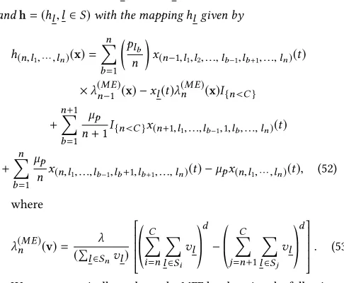
In Figure 2, by defining a processy(t,v)=(yn(t,v),0≤n≤C) referred to as the tail mean-field that satisfiesy(0,v) = vand
yj(t,v) = ÍC
i=jÍl∈Sixl(t,u), we plotϑtv(y(t,v),π∗) as a
func-tion oftwhereπ∗is the fixed-point ofy(t,v)andϑtvis the total variation distance defined by
ϑtv(w,z)= Õ
0≤n≤C
|wn−zn|. (56)
It is clear from Figure 1 and Figure 2 that the mean-fieldx(t,u) and its tail mean-fieldy(t,v)converge to their fixed-points for three different initial points whenλtakes 0.7 and 0.9. This supports that the mean-fieldx(t,u)andy(t,v)are globally stable.
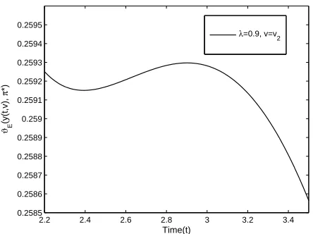
From Figure 2, it is clear thatϑtv(y(t,v),π∗)the total variation distance between the tail mean-fieldy(t,v)and its fixed-pointπ∗ is not monotonically decreasing. Further, letϑE(y(t,v),π∗)be the euclidean distance betweeny(t,v)andπ∗defined by
ϑE(w,z)=
s Õ
0≤n≤C
|wn−zn|2
. (57)
0 5 10 15 20 25 30 35 40
0 0.2 0.4 0.6 0.8 1 1.2
Time (t)
dtv
(x(t,u),
π
)
λ=0.7, u=u
1
λ=0.7, u=u2
λ=0.7, u=u3
λ=0.9, u=u1
λ=0.9, u=u
2
λ=0.9, u=u
[image:10.612.327.537.94.261.2]3
Figure 1: Convergence of the mean-field to its fixed-point
0 5 10 15 20 25 30 35 40
0 0.2 0.4 0.6 0.8 1 1.2 1.4 1.6
Time (t) ϑtv
(y(t,v),
π
*)
λ=0.7, v=v1
λ=0.7, v=v
2
λ=0.7, v=v
3
λ=0.9, v=v
1
λ=0.9, v=v2
[image:10.612.56.299.148.348.2]λ=0.9, v=v3
Figure 2: Convergence of the tail mean-field to its fixed-point
Then from Figure 3,ϑE(y(t,v),π∗)is also not decreasing mono-tonically. The case withλ=0.9 andv =v2for the region where
ϑE(y(t,v),π∗)is increasing is shown in Figure 4. Therefore from Figure 2 and Figure 3, both the total variation distance and the euclidean distance cannot be used for constructing a Lyapunov function to show the GAS of the tail mean-field.
[image:10.612.325.537.314.482.2]0 5 10 15 20 25 30 35 40 0
0.1 0.2 0.3 0.4 0.5 0.6 0.7
Time (t) ϑE
(y(t,v),
π
*)
λ=0.7,v=v1
λ=0.7, v=v
2
λ=0.7, v=v
3
λ=0.9, v=v1
λ=0.9, v=v2
λ=0.9, v=v
[image:11.612.64.277.94.262.2]3
Figure 3: Convergence of the tail mean-field to its fixed-point
2.2 2.4 2.6 2.8 3 3.2 3.4
0.2585 0.2586 0.2587 0.2588 0.2589 0.259 0.2591 0.2592 0.2593 0.2594 0.2595
Time(t) ϑE
(y(t,v),
π
*)
λ=0.9, v=v
2
Figure 4: Convergence of the tail mean-field to its fixed-point
in our analysis we assume that servers are sampled with replace-ment. By using PASTA property, we computeθN for various type of job length distributions by simulating the system up to 2000000 job arrivals. Letθ(exp)=(θ(exp)
i ,i ≥0)be the fixed point of the mean-field limit of the tail queue length process, then as shown in [32],
θ(exp)
i =
λ
µ
did−−1
1
. (58)
We now compute the total variation distance betweenθN and
θ(exp)defined as
ϑtv(θN,θ(exp))=Õ
i
θ
N i −θi(exp)
. (59)
We assume that the parametersλ,µ,dare fixed at 0.7,1, and 2, respectively. The different types of job length distributions that we
consider are exponential (Exp), constant (Const), power-law (PL), and mixed-Erlang (ME) distributions. The power-law distribution has CDFG(y) =1− 1
3y
3 2
fory ≥ 1
3 and zero otherwise. In the
mixed-Erlang case, the distribution hasi(1≤i≤2) exponential phases with probabilitypi and each exponential phase has rateµp. We choosep1 =.4,p2 =0.6 andµp is chosen by looking at the
formula of average job length given by
2 Õ
i=1
ipi
µp =
1
µ. (60)
[image:11.612.317.559.304.392.2]It is clear from Table 1 that for largeNsystem,θN for different job length distributions having same average job length can be approx-imated by the fixed-point of the mean-field limit under exponential job length distribution having the same average job length. This supports insensitivity and the global asymptotic stability of the mean-field limit.
Table 1:ϑtv(θN,θ(exp))for different job length distributions
N
Exp
Const
PL
ME
10
0.0424
0.0409
0.0419
0.0421
50
0.0078
0.0068
0.0072
0.0077
100
0.0060
0.0037
0.0071
0.0038
300
0.0012
0.0016
0.0016
0.0017
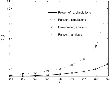
The SQ(d) policy even for small value ofdimproves the system performance significantly. We plot the average sojourn time (E(Ts)) of a job under the SQ(d) or Power-of-d policy and the random routing scheme (d=1) in Figure 5. The expression forE(Ts)under the SQ(d) or Power-of-dpolicy is given by
E(Ts)=Õ
i≥1
θiexp (61)
and for the random routing, we have
E(Ts)=Õ
i≥1 λ
µ
i
. (62)
We also plot the simulation results in Figure 5 by considering a system withN = 100 and exponential job length distributions. It is clear that the SQ(d) policy reduces the average sojourn time significantly over the random routing policy (d=1).
5.1
On the propagation of chaos in the
stationary regime:
We now discuss the relationship between the propagation of chaos in the stationary regime, the tightness of(πN)N, and the GAS of the equilibrium of the mean-field. For simplicity, we assume that the job length distributions are mixed-Erlang and each server has finite bufferC. Whenλ
µ <1, a finiteNsystem is stable[5], and hence there exists a unique invariant distributionπN for the Markov process
xN(t)=(xlN(t),l ∈S). In this case, the mean-field equations are
[image:11.612.55.277.319.485.2]0.1 0.2 0.3 0.4 0.5 0.6 0.7 0.8 0.9 1 2 3 4 5 6 7 8 9 10 11 λ E(T s ) Power−of−d, simulations Random, simulations Power−of−d, analysis Random, analysis
Figure 5: The average sojourn time (E(Ts)) versusλ
monotonicity properties unlike the simple exponential case and thus establishing propagation of chaos is a challenging problem as noted in [7]. When the GAS of the mean-field is true, by invoking Prokhorov’s theorem we can establish thatπN ⇒δπwhereπis the fixed-point of the mean-field[23]. This implies the validity of the interchange of limits
lim
N→∞
lim
t→∞x
N
t = lim
t→∞
lim
N→∞x
N
t . (63)
Further, this would then imply that propagation of chaos holds in the stationary regime[2, 23]. Thus it appears that GAS, propagation of chaos, and the coincidence of the stationary distribution and the fixed point of the mean field are all inter-related. We now discuss what happens when we cannot show GAS of the mean-field.
Since the space of probability measures onSdenoted byM1(S)
with metric induced by total variation distance is compact, from Prokhorov’s theorem[4], the sequence(πN)Nis tight inM1(M1(S))
under the topology induced by the weak convergence. Let(πNk)k be a converging subsequence with limiting pointZ∈ M1(M1(S)).
We say that for the sequence of systems with index(Nk)k, the limiting system is said to have stationary distributionZ for the stationary empirical random variable. Then form Theorem 1 of [2],
Zis an invariant distribution of the mean-fieldx(t,·)that means ∫
M1(S)
f(x(t,u))dZ(u)=
∫
M1(S)
f(u)dZ(u). (64)
Furthermore, from Theorem 3 of [3], the support ofZis a compact set included in the Birkhoff center of the mean-field where the Birkhoff center is the closure of the set of recurrent points. Hence the Birkhoff center includes the existing limit cycles, fixed-points of the mean-field.
LetqiNk(∞)be the random variable that denotes the state of serveriin the stationary regime in a finiteNksystem. LetVNk(∞),
V(∞)be random variables with distributionπNk andZ, respec-tively. Note that since the system behavior is symmetric to servers as servers’ labels do not play any role, the set(qNk
i (∞),1≤i≤Nk) is exchangeable irrespective of the initial conditions on(qNk
i (t),1≤
i≤Nk)in the transient regime. Let us consider continuous bounded mappingsϕi :S→ R+, 1≤i≤l.
Theorem5. IfπNk ⇒Z, then
E " l
Ö
i=1
ϕi(qiNk(∞))
#
→E
" l Ö
i=1
⟨V(∞),ϕi⟩
#
(65)
ask→ ∞. Any finite set of servers(ni)1≤i≤l in the limiting system of the sequence(πNk)k are mutually independent iffZis a Dirac
measure. Furthermore, ifZ =δafor somea ∈ M1(S), then each server state is a random variable with distributiona.
Proof. We can write
E " l Ö
i=1
ϕi
qNk
i (∞) # −E " l Ö
i=1
⟨V(∞),ϕi⟩
# ≤ E " l Ö
i=1
ϕi
qNk
i (∞) # −E " l Ö
i=1
⟨VNk(∞),ϕi⟩
# + E " l Ö
i=1
⟨VNk(∞),ϕi⟩
#
−E
" l Ö
i=1
⟨V(∞),ϕi⟩
# . (66)
Note that sinceVNk(∞) ⇒V(∞), the second term on the right hand side of the above inequality vanishes asNk→ ∞. Now, due to exchangeability, the permutation of states between servers does not affect the joint distribution. Hence, we have
E " l
Ö
i=1
ϕi
qNk
i (∞)
#
=
1
(Nk)lE
Õ
σ∈Q(l,Nk)
l
Ö
i=1
ϕi
qNk
σ(i)(∞)
(67)
where(N)j =N(N−1). . .(N−j+1), andQ(r,n)denotes the set of all permutations of the numbers{1,2, . . . ,n}takenrat a time. Also, by definition ofVNk(∞)we have
E " l
Ö
i=1
⟨VNk(∞),ϕi⟩
# =E © « l Ö
i=1
1
Nk Nk
Õ
j=1
ϕi
q(Nk)
j (∞) ª ® ¬ (68)
Hence, the first term on the right hand side of (193) can be bounded as follows E " l Ö
i=1
ϕi
qNk
i (∞) # −E " l Ö
i=1
⟨VNk(∞),ϕi⟩
#
≤2Bl
1−(Nk
)l (Nk)l
→0 asNk→ ∞
where maxi∥ϕi∥=B.
Finally, from equation (65), any finite set of servers are indepen-dent of each other iffZ is a Dirac measure. Otherwise they are coupled through the sample value of the random variableV(∞). If
witha. Then the following equation concludes that each server has distributiona
E " l
Ö
i=1
ϕi(qiNk(∞))
#
→
l
Ö
i=1
⟨a,ϕi⟩ (69)
asNk→ ∞. This completes the proof. □ SinceZis an invariant distribution of the mean-fieldx(t,·), from equation (64)
E " l
Ö
i=1
ϕi(qiNk(∞))
#
→
∫
u∈M1(S)
l
Ö
i=1
⟨x(t,u),ϕi⟩
!
dZ(u) (70)
asNk→ ∞. The equation (70) implies that in the stationary regime, at any timet, servers are coupled through the position of the mean-fieldx(t,·)which is a random element since its initial point is random with distributionZ. Furthermore, in the limiting system, at any instanttin the stationary regime, each servers’ state is a random variable with distribution coinciding with the position of the mean-field. For example, if support ofZcontains limit cycles or multiple fixed-points of the mean-field, then at any instant in the stationary, the position of the mean-field is random as a result, any finite set of servers are coupled.
5.2
Discussion on prior work in [6]:
In the literature, the only work that claims to prove the insensitivity of the stationary distribution of the limiting system is [6] based on anansatzthat we recall below. Using Theorem 5, we demonstrate that theansatzin [6] carries the necessary and sufficient conditions required to establish insensitivity of the limiting system. As a result, the insensitivity of the stationary distribution of a server state in the limiting system is an immediate consequence. Infact, theansatz is the result that we aim to establish in studying the large-scale systems under randomized load balancing in order to understand the impact of the load balancing policy on system performance by using the stationary distribution in the limiting system.
LetQN(t)=(r1,N(t),r1,N(t),· · ·,rN,N(t))is the joint queue-size process at timet whereri,N(t)(notationqi,n(t)is used in [6]) denotes the number of jobs at serveriat timet. LetΓN (Γis replaced withπin [6]) be the stationary distribution ofQN(t). We now recall exactly theansatzstated in [6].
Ansatz in [6]:
Demonstrate(ΓN) ⇒ (Γ)asN → ∞, whereΓis a stationary and ergodic measure onZ+∞. Show that the limitΓis unique, depending only on the service distribution, service discipline and load balancing rule. LetΓ(k)be the restriction ofΓto its firstkcoordinates, with
γ = Γ(1)
being the one-dimensional marginal ofΓ. Show that, for everyk,
Γ(k)=⊗k
i=1γ. (71)
LetQN(∞) =(QiN(∞),0 ≤i ≤C)whereQNi (∞)denotes the random variable in the stationary regime indicating the faction of servers withijobs. Then from Theorem 5 (also Proposition 2.1 of [12]),QN(∞) ⇒γwhereγ is a deterministic measure inM1(S). Since theSQ(d)policy uses the queue-size information of a finite set ofdrandomly sampled servers that have independent and identical distributions coinciding withγ, the arrival process is a Poisson
process to any particular server which is a necessary condition to have insensitivity in processor sharing systems. Furthermore, the arrival process to each server is a state-dependent Poisson arrival
process with rateλk =λ
(ÍC
j=kγj)d−(ÍC
j=k+1γj)
d
γk when there arek
jobs at the server. Therefore the set of arrival ratesΛ=(λk,0≤
k≤C)can be written as a function ofγas
Λ=F1(γ). (72)
Further, for given set of arrival ratesΛ, the stationary distribution for a server occupancy in the limiting system can be written through a mappingF2as
γ=F2(Λ). (73)
Thereforeγmust be an unique fixed-point of the mappingF2(F1)for
the case of general job length distributions which is not shown in [6] except for the case of FIFO queues with service time distributions having decreasing hazard rate functions. To have insensitivity,γ must be same for all the general job length distributions having same average job length. In [6], from uniqueness ofγ inansatz, insensitivity is concluded from reversibility since arrival process to each server is a state-dependent Poisson arrival process. Note that since the mappingsF2,F1are same for both exponential and general
distributions, the uniqueness of the fixed-point ofF2(F1)follows
from the GAS of the mean-field in exponential case. Therefore the fixed-point of the mappingF2(F1)is same for both exponential and
general job-length distributions when they have same average job lengths. Sinceansatzimplies the Poisson arrival process to servers and uniqueness of the stationary distribution in the limiting system, the insensitivity follows immediately. However, the proof ofansatz remains an open problem and has been shown only for the case of FIFO queuing models with service time distributions having decreasing hazard rate functions in [7].
6
CONCLUSIONS AND FUTURE WORK
In this paper we have obtained the mean-field limit for PS sys-tems under SQ(d) routing and have shown that its equilibrium point isunique and insensitive. In [6], the analysis was restricted to studying the limit limN→∞limt→∞νtN under the assumption of theansatz. Later [7], proved theansatz for the case of FIFO queuing models with service time distributions having decreasing hazard rate functions by exploiting the monotonic behavior of the system. However, as stated in [7, page 252] that the proof tech-niques cannot be extended to processor sharing models since the preordering of states is not possible unlike FIFO systems which is the key idea in showing monotonicity. On the other hand, the mean-field limit obtained by studying limN→∞νNt is a determinis-tic process. It is enough to show the GAS of the mean-field since the Prokhorov’s theorem would then imply the interchange of limits limN→∞limt→∞νNt = limt→∞limN→∞νNt . This will be addressed in future work.
REFERENCES
[1] R. Aghajani and K. Ramanan. 2017. The hydrodynamic limit of a randomized load balancing network.ArXiv e-prints(July 2017). arXiv:math.PR/1707.02005 [2] Michel Benaim and Jean-Yves Le Boudec. 2011. On Mean Field Convergence and
Stationary Regime. (11 2011).