warwick.ac.uk/lib-publications
Original citation:
Ambler, Michael, Vorselaars, Bart, Allen, Michael and Quigley, David (Researcher in physics).
(2017) Solid–liquid interfacial free energy of ice Ih, ice Ic, and ice 0 within a mono-atomic
model of water via the capillary wave method. The Journal of Chemical Physics, 146 (7).
074701.
Permanent WRAP URL:
http://wrap.warwick.ac.uk/86041
Copyright and reuse:
The Warwick Research Archive Portal (WRAP) makes this work of researchers of the
University of Warwick available open access under the following conditions.
This article is made available under the Creative Commons Attribution 4.0 International
license (CC BY 4.0) and may be reused according to the conditions of the license. For more
details see: http://creativecommons.org/licenses/by/4.0/
A note on versions:
The version presented in WRAP is the published version, or, version of record, and may be
cited as it appears here.
THE JOURNAL OF CHEMICAL PHYSICS146, 074701 (2017)
Solid–liquid interfacial free energy of ice Ih, ice Ic, and ice 0 within
a mono-atomic model of water via the capillary wave method
Michael Ambler,1Bart Vorselaars,1,a)Michael P. Allen,1,2and David Quigley1,b)
1Department of Physics, University of Warwick, Coventry CV4 7AL, United Kingdom
2H. H. Wills Physics Laboratory, Royal Fort, Tyndall Avenue, Bristol BS8 1TL, United Kingdom
(Received 8 November 2016; accepted 26 January 2017; published online 15 February 2017)
We apply the capillary wave method, based on measurements of fluctuations in a ribbon-like interfacial geometry, to determine the solid–liquid interfacial free energy for both polytypes of ice I and the recently proposed ice 0 within a mono-atomic model of water. We discuss various choices for the molecular order parameter, which distinguishes solid from liquid, and demonstrate the influence of this choice on the interfacial stiffness. We quantify the influence of discretisation error when sampling the interfacial profile and the limits on accuracy imposed by the assumption of quasi one-dimensional geometry. The interfacial free energies of the two ice I polytypes are indistinguishable to within achievable statistical error and the small ambiguity which arises from the choice of order parameter. In the case of ice 0, we find that the large surface unit cell for low index interfaces constrains the width of the interfacial ribbon such that the accuracy of results is reduced. Nevertheless, we establish that the interfacial free energy of ice 0 at its melting temperature is similar to that of ice I under the same conditions. The rationality of a core–shell model for the nucleation of ice I within ice 0 is questioned within the context of our results.©2017 Author(s). All article content, except where otherwise noted, is licensed under a Creative Commons Attribution (CC BY) license (http://creativecommons.org/licenses/by/4.0/).[http://dx.doi.org/10.1063/1.4975776]
I. INTRODUCTION
The crystallisation of ice I from liquid water continues to be a benchmark problem for molecular simulation. A variety of methods have been used to compute nucleation barriers.1–4 Homogeneous nucleation rates have been computed using the framework of classical nucleation theory5–7(CNT) or directly
with path sampling approaches.8,9 Heterogeneous nucleation
has been probed in a variety of studies.10–13
One particular subtlety presents a challenge to the accu-racy of molecular simulations. As yet no simulation has demonstrated a propensity for ice I to crystallise entirely in its hexagonal polytype ice Ih (ABABAB stacking of molecu-lar bilayers) at weak supercooling. Instead, simulations con-sistently produce stacking disordered mixtures of the cubic polytype ice Ic (ABCABC stacking) and ice Ih, as seen exper-imentally only at very low temperatures. The origin of this stacking disorder, and the preference for ordered hexagonal stacking in ice formed at weak supercooling, has been the subject of much discussion in the literature. For details, we refer the reader to a recent review by Malkinet al.14
In a recent communication, one of us (DQ) presented a thermodynamic argument that low temperature critical nuclei of ice I are most stable with stacking disordered structure.15
This model is based on nearest neighbour interactions between ice bilayers. In the context of nucleation from the liquid, rather than transformation from other ice phases, experiments
a)Current address: School of Mathematics and Physics, University of Lincoln,
Lincolnshire LN6 7TS, United Kingdom.
suggest that the stacking sequence is entirely random (no cor-relations involving more than three bilayers) and hence the nearest-neighbour approximation is reasonable.16At this level of approximation, any difference in solid–liquid interfacial free energy between cubic and hexagonal ice is neglected.
Historical experimental crystallisation data at low temper-ature can be interpreted as contradicting this assumption, based on CNT estimates for the interfacial free energyγc between cubic ice and supercooled water.17 Calculations ofγ
c from this data require a figure for the cubic–hexagonal free energy difference∆Gch. Calculations of this quantity are subject to considerable variation, ranging from a few J mol115 in the popular coarse-grained mW model18 to 627±300 J mol1 in first principles calculations with lattice vibrations treated anharmonically.19For any positive estimate of∆Gch, a value forγc, lower than the interfacial free energy between hexag-onal ice and water γh, is needed to explain the preferential nucleation of cubic ice within CNT.20Despite the likelihood that these historical experiments yielded stacking-disordered rather than pure cubic ice, the notion that variations in stack-ing sequence influence interfacial free energy is worthy of investigation.
One method for the calculation of solid–liquid inter-facial free energies from molecular simulation is via the analysis of capillary wave fluctuations.21–24This can require simulations on large length and time scales but is increas-ingly tractable. The method is implemented entirely via post-processing of simulation trajectories and does not require invasive modifications to simulation packages. Notably, such calculations have been largely confined to crystals with cubic symmetry; however Benet, MacDowell, and Sanz25 have
recently computedγhfor the popular TIP4P/200526atomistic model of water via this approach.
In the present work, our primary objective is to com-pute the solid–liquid interfacial free energy for both cubic and hexagonal ice in the mono-atomic mW model of water18
and to explore the factors which control and limit accu-racy of the capillary wave method when applied to ice–water interfaces. A recent study27using the “mold integration
tech-nique” provides a useful benchmark for comparison. This was unable to resolve differences in interfacial free energy between facets of ice Ih in the mW model or between the orientation-averaged γc andγh when using the TIP4P/Ice28 model. No comparison between the two polytypes was made for the mW model.
The mW model represents the water molecule with a Stillinger–Weber type potential, favouring tetrahedral local environments and parametrised to capture structural and ther-modynamic properties of the ice–water system. The model has been used in a number of ice nucleation simulations, in all cases leading to crystallites of mixed cubic and hexagonal character.3,8,29,30This model represents an interesting case, as
the difference in bulk stability between cubic and hexagonal ice is very small.15 This leads to the expectation of stack-ing disordered nuclei atalltemperatures where homogeneous nucleation is achievable, should the assumption thatγh ≈γc hold.
In a recent work, Russo, Romano, and Tanaka31 have obtained an improved CNT fit to low-temperature nucleation simulations (also using the mW model) by including a low den-sity metastable ice phase (ice 0) as the first nucleated species within a 3 parameter core–shell nucleation theory. The inter-facial free energyγzbetween ice 0 and water is wrapped into one of these fitting parameters and must be somewhat lower than bothγh andγc to offset the lower bulk stability of ice 0.32 As a secondary objective, we compute the interfacial
free energy between ice 0 and water directly and determine how this influences the interpretation of the core–shell fit in Ref.31.
II. METHODS
Our calculations closely follow the method of Hoyt, Asta, and Karma,33 which has been mainly used to cal-culate the solid–liquid interfacial free energy for crystals with cubic symmetry.21–24 The interfacial free energy is dependent on the crystallographic surface exposed to the melt and can be represented as a function on the unit sphere,
γ(θ,ϕ)=γ01+1S1(θ,ϕ)+2S2(θ,ϕ)+. . .. (1)
Here the functions Si represent a basis set of symmetry-adapted spherical harmonics appropriate to the point group of the solid crystal. Provided the free energy is only weakly anisotropic, the symmetry adapted nature of these functions ensures that the series can be truncated after the first few terms. In the case of crystals with cubic symmetry, the appro-priate basis functions are the Kubic harmonics. In the general case, generation of appropriate functions in a suitable form is non-trivial. Implementation of an automated method for
doing so, with only the crystallographic unit cell as input,34 is available via the “gencs” utility distributed with the Alloy Theoretic Automated Toolkit (ATAT).35This enables
applica-tion of the capillary wave method to a much wider range of systems. Appropriate functionsSifor cubic and hexagonal ice I, and for ice 0, are given in the supplementary material as Equations (S3)–(S5).
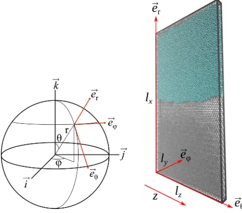
As the interfacial free energy cannot be determined directly from simulations, the coefficientsiare obtained via fitting to multiple measurements of the interfacialstiffnessγ˜ along directions in the tangent plane perpendicular to the sur-face normal (see Figure 1). The stiffness along a particular direction ˆuin the tangent plane is related to the interfacial free energy via33
˜
γ(θ,ϕ, ˆu)=γ(θ,ϕ)+uˆTHγ(θ,ϕ) ˆu, (2)
whereHγ(θ,ϕ) is the Hessian matrix (in polar coordinates) expressing the second derivatives of γ(θ,ϕ) evaluated at anglesθandϕ.
The stiffness itself is computed via simulation of a “ribbon-like” interfacial geometry along ˆu, under conditions of equilibrium coexistence. With reference to the example geom-etry in Figure1, the interface is divided intoNz columns of widthδz, centred on discrete valueszn, containing an element of solid–liquid interface of area δA = lyδz. In each column the quantityh(zn) is computed, indicating thexposition of the interface relative to its mean position.
Following earlier authors,24 we denote the simulation setup via the Miller indices of the (hkl) crystallographic plane exposed to the liquid and the direction [h0k0l0] along which the simulation box is shortest (the y direction in Figure1). For example, a simulation geometry for the (110) surface of cubic ice in which the short direction is taken as [001] will be denoted as (110)[001].
[image:3.594.308.546.490.699.2]When comparing solid-liquid interfacial free energies between two crystal structures, it is important to calculate
FIG. 1. Simulation geometry. Cartesian vectors~i,~j, and~kdenote the crystal coordinate system such that the polar anglesθandϕdefine a surface normal. Molecular dynamics simulations are performed in a local coordinate system with thexdirection chosen along this normal. In this case, the direction ˆu=~eθ
074701-3 Ambleret al. J. Chem. Phys.146, 074701 (2017)
interfacial height profiles with the same choice of local order parameter ξ, used to locate the x position of the interface and hence h(zn) in each column. For the cubic ice Ic struc-ture, the commonly used q6 order parameter performs well but recognises only three solid neighbours in ice Ih leading to an erroneous large difference between the interfacial free energies of these two polytypes.
A better choice, which is appropriate for ice I interfaces only, is the CHILL+ algorithm of Nguyen and Molinero.36 This is based on the ubiquitous Steinhardt order parameter.37 A per-molecule vector~q3 is constructed with 7 components, each of which is a sum of the l = 3 spherical harmonics calculated for the unit vectors connecting a molecule to its four nearest neighbours. The correlation of~q3between each molecule and its neighbours is used to classify molecules as solid, liquid, or interfacial. We refer readers to Ref. 36 for details and note that a very similar order parameter was used to construct a reaction coordinate for ice nucleation in earlier work.8 In our work, we assign ξ = 10 to molecules
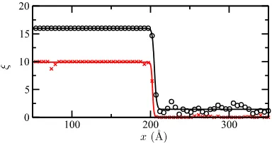
identi-fied as ice-like by CHILL+,ξ =0 to molecules identified as liquid, andξ = 5 to molecules (if any) identified as interfa-cial. We then plot (as a function ofx) the quantity ¯ξas the average value ofξ over all molecules within each of theNx elements of width δxalong the column perpendicular to the area elementδA. A tanh function is then fitted to these data and thex position of the interface is taken as the inflexion point.
To assess any variability of results arising from the choice of local order parameters, we also compute the interfacial position using the more complex order parameter of Russo, Romano, and Tanaka.31 This order parameter is also able to distinguish ice 0 from liquid. Here the vector order param-eter ~q12 is used, accumulated over the 16 nearest neigh-bours of each molecule. The vector~q12 for each molecule is then replaced with the average over these 16 neighbours. Molecules are deemed to be connected if the dot product of their respective normalised ~q12 vectors exceeds a threshold value of 0.75. Here we setξequal to the number of such con-nections on each molecule and locate the interface by fitting
¯
ξ as a function of x to a tanh function as above. Example data for both methods of locating the interface are shown in Figure 2. An example interfacial height profile is shown in Figure3.
FIG. 2. Plot of the averaged local order parameter ¯ξfor particles within vol-ume elements running along columns perpendicular to an ice 1c (111)[1¯10] interfacial ribbon geometry. Red crosses indicate ¯ξcomputed via the CHILL+ algorithm and black circles via the~q12connections. Solid lines are tanh fits
to the data, identifying the location of the interface as the point of inflexion at
[image:4.594.309.547.48.173.2]x= 205.0 Å (black line) andx= 202.6 Å (red line).
FIG. 3. Interface location in the ice Ic (111)[1¯10] geometry. The computed interface shape is plotted as red points, each of which indicates the inter-facial position at each of 50 discretised points in the z direction. Water molecules are coloured according to their number of solid-like connec-tions, in this case identified via the~q12 order parameter. Particles with
more than 12 connections are coloured grey, with the remainder coloured turquoise. Red beads mark the position of the interface (also identified by
~q12) in each interfacial column. System dimensions are those reported in
TableI.
It is apparent that the two order parameters identify inter-facial positions which can differ by an amount comparable to the intermolecular spacing in the crystal. Should this dif-ference prove to be anything but a constant offset, then the shape ofh(zn) (and hence the calculation of the interfacial free energy) will be order-parameter dependent. We investigate this explicitly in SectionIV.
For small wavenumbersq, the discrete Fourier transform h(qn) of these profiles can be connected to the interfacial stiffness via
h|h(qn)|2i= kBT
Aγ˜q2 n
, (3)
whereA = lylz is the interfacial area. By plotting measure-ments of this quantity againstqnon a double logarithmic scale, one obtains a linear plot from which the interfacial stiffness can be extracted from the intercept. The requirement of small wavenumber restricts linear behaviour to small values ofqnδz such that sin (qnδz) ≈ qδz.22 In our work, we restrict the linear fit to modes for whichqnδz < 0.5. We also note that Equation(3)is dependent on the interfacial ribbon having a width sufficiently small that no energy is present in modes along the short orydirection in Figure1. For facets with large surface unit cells, that requirement may be difficult to rec-oncile with that of surface periodicity, leading to a spurious dependence of the measured stiffness on the ribbon widthly.
We calculate ˜γ for two mutually orthogonal choices of the surface direction ˆu at each of the several surface planes, averaging the resulting stiffness when these are equivalent by symmetry. The coefficients (γ0,1,2. . .) are then chosen to minimise the total difference between the measured stiff-ness values and those obtained by substituting Equation (1)
into(2). For further details of the method we refer the reader to Ref.21.
[image:4.594.71.263.587.688.2]the enthalpy is conserved to within fluctuations of the barostat kinetic energy. This has the advantage of constraining the long-term average solid fraction via a feedback mechanism between latent heat and temperature. The three cell dimensionslx,ly, andlzwere allowed to vary independently subject to constant 90◦cell angles. This ensures that the interface is unstrained at
all points of the feedback cycle. All simulations used a time step of 1 fs. Simulations of ice I interfaces were conducted at the mW melting temperature using 30 000–50 000 molecules with an interfacial ribbon of length 180–200 Å. Ice 0 simu-lations required substantially larger ribbon lengths to capture sufficient wavevectors for accurate fitting. In this case simu-lations used 80 000–180 000 molecules at the ice 0 melting temperature of 240 K, with ribbon lengths of 570–620 Å.
III. GEOMETRY AND CONVERGENCE
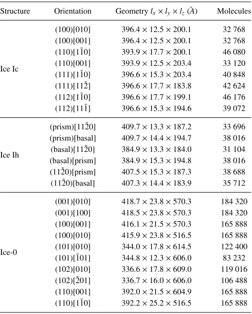
TableIreports the simulation geometries used in recon-structing the interfacial free energy of all three ice structures. In this section, we carefully consider the convergence of the measured interfacial stiffness for example surfaces. We exam-ine how the spatial resolution at which the interfacial ribbon is sampled and the simulation run length govern accuracy of stiffness measurements. We also establish how the width of the ribbon (y direction in Figure 1) influences stiffness measurements.
A. Spatial resolution
We first consider convergence with respect to the spa-tial sampling resolutionδz along the interfacial ribbon. It is
TABLE I. Interfacial geometries used in calculating the stiffness of ice–water interfaces leading to reconstruction of the anisotropic interfacial free energy.
Structure Orientation Geometrylx×ly×lz(˚A) Molecules
Ice Ic
(100)[010] 396.4×12.5×200.1 32 768 (100)[001] 396.4×12.5×200.1 32 768 (110)[1¯10] 393.9×17.7×200.1 46 080 (110)[001] 393.9×12.5×203.4 33 120 (111)[1¯10] 396.6×15.3×203.4 40 848 (111)[11¯2] 396.6×17.7×183.8 42 624 (112)[1¯10] 396.6×17.7×199.1 46 176 (112)[11¯1] 396.6×15.3×194.6 39 072
Ice Ih
(prism)[11¯20] 409.7×13.3×187.2 33 696 (prism)[basal] 409.7×14.4×194.7 38 016 (basal)[11¯20] 384.9×13.3×184.0 31 104 (basal)[prism] 384.9×15.3×194.8 38 016 (11¯20)[prism] 407.5×15.3×187.3 38 688 (11¯20)[basal] 407.3×14.4×183.9 35 712
Ice-0
[image:5.594.308.550.47.186.2](001)[010] 418.7×23.8×570.3 184 320 (001)[100] 418.5×23.8×570.3 184 320 (100)[001] 416.1×21.5×570.3 165 888 (100)[010] 415.9×23.8×516.5 165 888 (101)[010] 344.0×17.8×614.5 122 400 (101)[¯101] 344.8×12.3×606.0 83 232 (102)[010] 336.6×17.8×609.0 119 016 (102)[¯201] 336.7×16.0×606.0 106 488 (110)[001] 392.0×21.5×604.9 165 888 (110)[1¯10] 392.2×25.2×516.5 165 888
FIG. 4. Interfacial stiffness calculated via Equation(3)as a function ofNzfor
three interfacial geometries. System dimensions are those reported in Table
I. Red points indicate calculations using height profiles computed via the CHILL+ algorithm and black via the~q12solidity criterion.
important to note two distinct effects of this parameter. Smaller
δz leads to a more accurate representation of the interface geometry but also affords a larger maximum wavevector to be included in fitting Equation(3).
Figure 4plots the stiffness measured for a selection of interfacial geometries as a function of Nz when including all wavevectors q for whichqδz is less than 0.5. Jumps in stiffness are observed at values ofNzfor which new wavevec-tors commensurate with the periodicity of the simulation box become available. Convergence to within statistical uncer-tainty is achieved at Nz = 50 for both ice I polytypes, and atNz = 100 for ice 0, which for both cases corresponds to a
δzclose to interatomic spacing. We note that in the case of ice 0, sampling withNz= 20 leads to a stiffness less than half the converged value.
Figure5plots the measured stiffness versusNzfor the ice Ih (basal)[11¯20] geometry at afixednumber of wavevectors. Comparison with the central panel of Figure4indicates that enhanced resolution in the representation ofh(zn), rather than inclusion of additional wavevectors in the analysis, has the greater effect on convergence.
[image:5.594.44.289.443.748.2]Figure 5 also shows the effect of spatial resolution in the direction normal to the interface, demonstrating that a sufficiently high Nx must be used to accurately capture the
FIG. 5. Interfacial stiffness as a function ofNzat fixedNx = 80 (left) and
as a function ofNx at fixedNz= 50 (right). In both cases, the simulation
geometry is ice Ih (basal)[11¯20]. Simulation dimensions are those reported in TableI. Red points indicate calculations using height profiles computed via the CHILL+ algorithm and black via the~q12solidity criterion. In all cases, ˜γ
[image:5.594.313.543.556.687.2]074701-5 Ambleret al. J. Chem. Phys.146, 074701 (2017)
interfacial heighth(zn) and hence the stiffness. Errors intro-duced by insufficient resolution alongzandxare similar in magnitude but of opposite sign. Sampling at very close to the ultimate limit of spatial resolution (the interatomic spacing) is required to achieve converged results. We adopt the strategy of sampling at as close to this limit as possible for the remainder of this paper.
B. Thickness of interfacial ribbon
The standard analysis which leads to Equation(3)assumes a pseudo-one-dimensional geometry in which the width of the interfacial ribbon ly is assumed to be sufficiently thin that no energy is present in fluctuations along y. For the lowest index surfaces of crystals with cubic or orthorhombic sym-metry, very thin interfacial ribbons can easily be constructed in the geometry of Figure 1 for which ly is commensurate with the periodicity of the surface unit cell. For higher index surfaces, or for crystals (such as ice Ih) with non-orthogonal symmetry, undesirable (for purposes of analysis) skewed sim-ulation cells are required to achieve the minimum possible ribbon thickness. In practice, one normally accepts a thicker ribbon to achieve orthogonal supercells and to satisfy the min-imum image convention for efficiency. The effect of using these larger ribbon thicknesses has been explored previously in the context of aluminium22 but never (to our knowledge)
for ice.
To establish a benchmark property of a flat solid–liquid interface, we simulate the ice Ih (basal)[prism] geometry using a reduced cross section of ly = 13.3 Å, lz = 15.4 Å, over a sufficiently short period of time that capillary waves are not observed. The root mean square deviation (RMSD) of the interfacial height profile in this simulation is measured as 0.69(8) Å, which we take as the reference value for an atomically “flat” interface, i.e., the minimum possible devia-tion from a constant interfacial height resulting from thermal fluctuations of the atomic position about their lattice sites only.
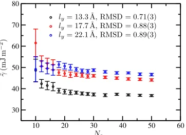
[image:6.594.77.258.543.675.2]In Figure6we plot the convergence of the interfacial stiff-ness as a function ofNzfor three thicknesses of the interfacial ribbon in the ice 1h (basal)[prism] geometry. In each case, we
FIG. 6. Calculated interfacial stiffness as a function ofNzfor three
thick-nesses of the interfacial ribbon in the ice Ih (basal)[11¯20] geometry. Other dimensions are as reported in TableI. The RMS deviation from a perfectly uniform profile across the interfacial ribbon (ydirection in Figure1) is also indicated. The RMSD for a “flat” surface is 0.69(8), indicating that forly
= 13.3 Å no capillary waves are present in theydirection. The interface position is located via the~q12solidity criterion.
further divide each discrete interfacial element into sections of width δyand measure the RMSD from the mean height profile over these sections. The resulting quantity can be com-pared to the value of 0.69(8) Å to establish if the geometry is sufficiently narrow to suppress capillary waves across the rib-bon. An appreciably different stiffness is observed for the nar-rowest ribbon, which is the only geometry in which the above criterion is satisfied. For thicker ribbons, the presence of energy in modes across the ribbon results in an overestimate of the pseudo-one-dimensional stiffness.
As the stiffness of ice I solid–liquid interfaces is expected to be approximately isotropic, we adopt the strategy of keeping the interfacial ribbon at this thickness or smaller, while remain-ing sufficiently wide to avoid the self-interaction of molecules with their periodic images. For ice 0, this is problematic. The tetragonal unit cell of ice 0 results in larger minimum ribbon thicknesses even for low index interfaces due to periodicity constraints. Furthermore, as the interfacial stiffness of this phase is expected to be lower, one expects the criteria for the suppression of capillary waves across the ribbon to impose a narrower geometry than that for ice I. We must therefore acknowledge that for the ice 0 system sizes reported in TableI, the resulting stiffness and free energy estimates represent an upper bound.
C. Simulation length
[image:6.594.322.537.551.689.2]Each measurement of stiffness should be made over a sufficient number of fluctuations to accurately represent the ensemble of interfacial height profiles in the current geometry. In Figure7we plot the convergence of the interfacial stiffness as a function of time for representative geometries of ice Ic, ice Ih, and ice 0. In the case of ice I phases, the interfacial stiff-ness measurement is converged to within statistical error after approximately 80 ns of simulation. In the case of ice 0, where the use of largerlzleads to additional spatial averaging, con-vergence is achieved at approximately 25 ns. For all interfacial geometries, we carefully ensure that the stiffness measurement is converged with respect to the simulation length to a similar accuracy.
FIG. 7. Calculated interfacial stiffness as a function of simulation time. The left panel plots the stiffness for the ice Ih (basal)[11¯20] (black) and the ice Ic (111)[1¯10] (red) geometries which expose identical crystal layers to the liquid. The right panel shows much more rapid convergence for the ice 0 (001)[010] system. The interface position is located via the~q12solidity criterion in all
IV. RESULTS
We simulate ice–water interfaces for a number of surfaces corresponding to large interplanar spacingsDhkl, these being expected to have the lowest interfacial free energy and hence be most commonly expressed in the crystal morphology.41
A. Ice Ih
Plots from which the stiffness of ice Ih interfaces were extracted are shown in Figure 8 for the case where the interface was located using the~q12solidity criterion. All plots should share a common gradient of −2 on the logarithmic scales shown, which is applied as a constraint in the fitting procedure.
When fitting these data to second derivatives of Equation(1), we find that the contribution from the term in §2 is negligible. Any improvement upon including eitherS3 and/orS4is marginal. The best fit is achieved when including the isotropic term plusS1andS4only, constraining2and3to zero. This suggests that the weak deviations from an isotropic interfacial free energy are almost entirely captured via theS1 term.
[image:7.594.305.551.92.169.2]Details of the optimised parameters and the fitted versus measured stiffnesses are reported in Tables S1, S4, and S7 of thesupplementary material.
FIG. 8. Logarithmic plots of the average Fourier-transformed interface height squared weighted by the areaAdivided by thermal energykBTas a function
ofqfor various simulations of interfaces between ice Ih and water. Solid lines are a linear fit to the data points satisfyingqδz<0.5. In this case, the~q12
[image:7.594.310.548.293.695.2]solidity criterion is used to locate the interface.
TABLE II. Interfacial free energy at each of the three ice Ih surfaces studied. Results are reported for both the CHILL+ and~q12methods of locating the
solid–liquid interface. Results obtained by Espinosa, Vega, and Sanz27using
the mold integration technique are shown for comparison.
γh(mJ m2)
Method (Prism) (Basal) (11¯20) CHILL+ 35.2(2) 33.0(2) 35.3(2)
~q12 36.8(3) 34.4(4) 36.9(3)
Mold integration27 35.1(8) 34.5(8) 35.2(8)
The final estimates of interfacial free energy for ice Ih at coexistence are given in TableII, where the results of Espinosa, Vega, and Sanz27computed via the mold integration technique
are shown for comparison.
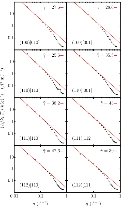
B. Ice Ic
Plots from which the interfacial stiffnesses of ice Ic were extracted are shown in Figure9.
FIG. 9. Logarithmic plots of the average Fourier-transformed interface height squared weighted by the areaAdivided by thermal energykBTas a function
ofqfor various simulations of interfaces between ice Ic and water. Solid lines are a linear fit to the data points satisfyingqδz<0.5. In this case, the~q12
[image:7.594.48.287.359.697.2]074701-7 Ambleret al. J. Chem. Phys.146, 074701 (2017)
TABLE III. Calculated solid–liquid interfacial free energies of all ice Ic sur-faces considered in this work. Results are shown for both methods of locating the solid–liquid interface when includingmparameters (m−1 symmetry adapted functions) in the fit to ˜γc(θ,ϕ).
γc(mJ m2)
m= 3 m= 4 m= 5
Plane CHILL+ ~q12 CHILL+ ~q12 CHILL+ ~q12
(100) 33.4(2) 35.4(3) 34.6(2) 37.3(3) 34.6(2) 37.2(3) (110) 32.7(2) 34.7(3) 33.8(2) 36.6(3) 33.8(2) 36.4(3) (111) 32.1(2) 33.9(3) 33.2(2) 35.9(3) 33.2(2) 35.7(3) (112) 32.5(2) 34.4(3) 33.5(2) 36.2(3) 33.5(2) 36.0(3)
When fitting these data to second derivatives of Equation (1), we find a systematic improvement in the fit when including terms up to and including S3. Including the S4term leads to no discernible change to within the statistical uncertainty of the resulting interfacial free energies. Calculated interfacial free energies for the four ice Ic interfaces studied are presented in TableIII.
Details of the optimised parameters and the fitted versus measured stiffnesses are reported in Tables S2, S5, and S8 of thesupplementary material.
As with ice Ih, interfacial free energies calculated via the use of the~q12solidity criterion are systematically higher than those obtained via CHILL+. There is no significant difference in the overall magnitude of the free energy between the two polytypes. The (111) plane of ice Ic and the basal plane of ice Ih expose identical surface structures to liquid up to the second sub-surface ice double-layer. Within our calculations, the free energies of these two surfaces are identical to within statistical error for the CHILL+ order parameter but differ by a small but measurable amount when using~q12.
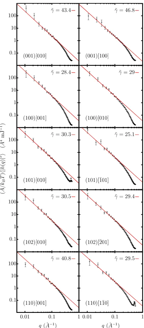
C. Ice 0
Plots from which the interfacial stiffnesses of ice 0 were extracted are shown in Figure10. Note that results are calcu-lated using only the~q12method of identifying the solid–liquid interface, as CHILL+ does not usefully recognise ice 0 as a solid.
Fitting the measurement stiffnesses to second deriva-tives of Equation(1) retained terms up to and includingS5. Details of the optimised parameters and the fitted versus mea-sured stiffnesses are reported in Tables S3, S6, and S9 of the
supplementary material. Fitted interfacial free energies for ice 0 are presented in TableIV.
V. DISCUSSION
A. Ice Ih
We first discuss our results for the interfacial free energy of ice Ih in comparison to the mold integration calculations of Espinosa, Vega, and Sanz27for the mW model. Both our methods of identifying the solid–liquid interface consistently lead to a small but measurable anisotropy in estimates ofγh favouring the basal plane, a feature not evident in the mold integration results. While the statistical uncertainty in our esti-mates is smaller, there is a systematic difference between our
two sets of data, the~q12 order parameter leading to slightly higher interfacial free energies at all surfaces. We note that the mold integration method doesnotrequire an order param-eter for identifying molecules which lie within a solid-like environment, which from these results would appear to be a source of small but significant systematic error in capillary wave calculations.
The fitted isotropic componentγ0 =34.5(2) mJ m2 for the CHILL+ solid identification and 36.0(3) mJ m2 when
FIG. 10. Logarithmic plots of the average Fourier-transformed interface height squared weighted by the areaAdivided by thermal energykBTas
a function ofqfor various simulations of interfaces between ice 0 and water. Solid lines are a linear fit to the data points satisfyingqδz< 0.5. The~q12
[image:8.594.313.546.165.696.2]TABLE IV. Calculated solid–liquid interfacial free energy for all planes of ice-0 considered in this work.
Plane (001) (100) (101) (102) (110)
γz(mJ m2) 31.3(5) 35.2(5) 34.6(4) 33.6(4) 34.2(4)
using~q12. These bracket the value of 35.5(3) mJ m2obtained by Espinosa et al.7 for the mW model when extrapolating results of the seeding method to coexistence.
Despite these small systematic differences from earlier work, our results confirm that the ice Ih–water interfacial free energy for the mW model lies toward the upper end of the experimental estimates and is somewhat higher than values obtained with detailed atomistic models.7,25
B. Ice Ic
We now compare values of interfacial free energy between the two ice I polytypes. When using the CHILL+ method of identifying the solid–liquid interface, the (111) face of ice Ic and the basal plane of ice Ih have identical interfacial free energies to within the statistical uncertainty of our measure-ments and fits. It might be expected that these two surfaces are both perpendicular to the stacking direction and hence present identical molecular arrangements to the liquid within the first two bilayers. Hudaitet al.30 have recently demonstrated by other methods that the surface tension of these two surfaces is identical. In our work, the~q12method of identifying the solid– liquid interface resolves a slight difference in interfacial free energy between these two surfaces; however, this difference is smaller than the discrepancy between the two choices of order parameter and cannot be considered significant. We also note that the isotropic component of the interfacial free energyγ0 is identical to within statistical uncertainty between the two polytypes when using~q12 (Tables S4 and S5 of the
supple-mentary material), but there is a small systematic difference in this quantity when using CHILL+. Again this is smaller than the difference in interfacial free energy measured by the two choices of order parameter.
We therefore conclude, to within the error inherent in the choice of order parameter and finite sampling of the interfa-cial fluctuations, that the interfainterfa-cial free energies of cubic and hexagonal ice I should be considered identical within the mW model. We have not considered the interfacial free energy of surfaces formed by stacking disordered ice but would expect this to be indistinguishable from the pure polytypes given the above results.
C. Temperature dependence ofγfor ice I
The capillary wave method is limited to measurements of interfacial free energy at the melting temperature. Here the area of an infinite plane interface is well defined by the geometry of the simulation cell. As recently discussed by Cheng, Tribello, and Ceriotti,42awayfrom coexistence the par-titioning of nucleus free energy into volume and surface area terms is essentially arbitrary. If one chooses (as in the seeding method) to calculate the volume contribution as the number of molecules n in the solid nucleus multiplied by the bulk chemical potential difference between solid and liquid, then
the resultingγwill depend on the interfacial area and hence how one chooses to define the (usually spherical) dividing sur-face. To be consistent with the usual assumptions of CNT, this surface should be chosen such that the enclosed volume is V =ρsn, whereρsis the number density of molecules in the bulk solid. Cheng, Tribello, and Ceriotti42further demonstrate
that imposition of this criterion is equivalent to the Tolman curvature correction toγ.
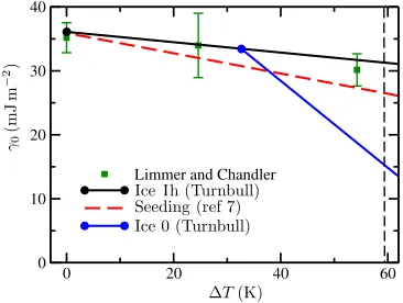
We note here that the seeding method calculations of Espinosaet al.7are necessarily consistent with CNT by design and use only data at the critical nucleus size. The resulting fitted interfacial free energies are Tolman-corrected for the curvature of the critical nucleus, the size of which is temperature depen-dent. In Figure11we compare these data to interfacial free energies extrapolated from our measurements via the Turnbull correlation,44,45
γ0(T)=C∆H(T)ρ2s/3(T), (4)
where∆H(T) is the temperature dependent enthalpy difference between solid and liquid andC is a constant determined by our measurement ofγ0at coexistence. We use measurements of∆H(eV/molecule) and ρs (molecules per cubic angstrom) readily obtained via straightforward simulation. Here we use the isotropic component ofγh(in mJ m2) computed using the
~q12order parameter for comparison to ice 0 in Sec.V D. In these units, this leads to a Turnbull coefficient ofC= 38.5. In all cases, the fittedγ0(T) obtained via the seeding method cal-culations of Espinosaet al.7 lies below that estimated from the Turnbull correlation, consistent with a positive Tolman length and a lowering of the interfacial free energy as expected for ice nuclei.46Furthermore, the magnitude of the difference increases with decreasing temperature, i.e., in inverse propor-tion to the critical nucleus radius of curvature. We conclude that the Turnbull correlation is useful in extrapolating inter-facial free energies away from coexistence, provided that the resulting data are interpreted as lacking the Tolman correc-tion. This is consistent with the work of Limmer and Chan-dler43who compute planar interfacial free energies away from
FIG. 11. Isotropic component of the solid–liquid interfacial free energy for ice Ih and ice 0 as a function of the temperature below freezing of ice I. Tem-perature dependence is extrapolated from calculations at coexistence (solid dots) via the Turnbull correlation. The values fitted to simulations of seeded ice Ih critical nuclei by Espinosaet al.7are shown for comparison, as are calculations of ice I planar interfacial free energies by Limmer and Chan-dler.43The dashed line indicates the temperature at which Russo, Romano,
[image:9.594.337.520.531.669.2]074701-9 Ambleret al. J. Chem. Phys.146, 074701 (2017)
coexistence and favourably compare these to predictions from the Turnbull correlation.
It should be noted that improved fits to explicitly com-puted nucleation barriers have been reported when allowing the solid–liquid chemical potential difference to deviate from the bulk value, both for mW ice3and simple lattice models,47
i.e., a value of γ0 consistent with the usual assumptions of CNT may not be optimal.
D. Core–shell model for nucleation of ice 0
We now turn our attention to the results for ice 0 inter-faces. Our results indicate an anisotropic interfacial free energy which would lead to non-spherical crystallites slightly com-pressed along thec-axis. Espinosaet al.48have recently
cal-culated a value for γz = 35.5 mJ m2 at the ice 0 melting temperature using mold integration. Details of the exact sur-face used are not given; however, this figure is remarkably consistent with our calculation at the (100) surface.
As calculated in Ref.32, the value ofγzneed only be 10% lower thanγhin order for the barrier to ice 0 nucleation to be smaller than for ice I. Russo, Romano, and Tanaka31interpret this preferential nucleation via a modified CNT in which nuclei have an internal ice I core structure coated in a shell, thickness
∆R, of interfacial ice 0. Forsmallwidths of the outer shell, this reduces to the following form of free energy∆Fof a growing nucleus relative to the metastable liquid,
β∆F(n)=an+bn2/3+cn1/3, (5)
where n is the number of particles within the growing ice I nucleus and β is the inverse temperature. The quantityγz appears in bothbandc, which were treated as fitting param-eters in Ref. 31. By repeating the fit of Equation (5) to the measuredF(n) data reported in Ref.31at 215.2 K, we obtain a=−0.134,b= 0.120, andc= 7.404.
Within this interpretation, one can reasonably neglect the Tolman correction when comparingγhtoγzas the radii of cur-vature for the ice 0 shell and the competing pure ice I nucleus are similar. Figure 11includes the temperature dependence of the isotropic component γ0 of the interfacial free energy between ice 0 and liquid water, extrapolated via the Turnbull correlation as for ice I. For ice 0, the Turnbull coefficient using the same units as above isC= 312, very much larger than for ice I. This is due to the much smaller difference in enthalpy between solid and liquid at coexistence. Consequently, the gra-dient ofγz(T) is much steeper than for ice I. At 215.2 K it is clearly energetically favourable to form a liquid interface to ice 0 rather than to ice I.
Using the data from Figure11and other thermodynamic parameters as used in Refs.15and32, the CNT barrier heights to the nucleation of ice 0 and ice I are very similar (within a few percent) at 215.2 K, suggesting ice 0 nucleation is at worst an energetically competitive crystallisation route in the mW model. Explicit calculations ofγaway from coexistence would be required to draw definitive conclusions which do not rely on the empirical Turnbull correlation.
It is however informative to revisit the above fit to a core– shell nucleation model using our extrapolated value forγzat 215.2 K. The thickness of the ice 0 shell is related to the fitting
parametercby the relationship
∆R= 3
2/3c
24βπγz
(4π ρs)1/3, (6)
whereρsis the number density of molecules in the ice I core. Constraining the interfacial free energy between ice 0 and water to that in Figure11requires that the shell thickness∆Ris 3.3 Å. Only slightly larger values would result from Tolman-corrected values ofγz. We must acknowledge that our ice 0 results should be interpreted as an upper-limit onγzdue to the use of large interfacial ribbon widths, more accurate results may increase the calculated shell thickness further. Based on the trend for ice I in Figure6, we suggest that this could not increase the shell thickness by a factor of two, required to accommodate the smallest unit cell dimension of ice 0. We suggest that the improved fit to nucleation data obtained in Ref.31is a result of the extra degree of freedom in the fitting procedure rather than an indication of core–shell behaviour.
In addition to their mold integration calculations at the mW ice 0 melting temperature, Espinosa et al.48 have also used simulations seeded with spherical nuclei to calculate the nucleation rate of pure ice 0 crystallites at a higher temperature of 226.5 K. We note that the use of spherical crystallites in that work may under-represent the lower energy (001) interface of ice 0. At this temperature, the isotropic estimate ofγzwas cal-culated as 29.9 mJ m2, leading to a nucleation rate 200 orders of magnitude lower than that for ice Ih under the same condi-tions. This value ofγzis indeed higher than that predicted by our calculations, as would be expected for spherical nuclei, but (as discussed above) implicitly contains a Tolman correction for the critical nucleus size which would be expected to act against such a difference. We cannot conclusively state that the use of non-spherical nuclei in seeding calculations would lead to a higher nucleation rate for ice 0.
Taken in isolation, our results do not rule out the nucle-ation of pure ice 0 crystallites at very low temperatures in the mW model; however, we rely on use of the Turnbull correlation which has not been validated by other methods for ice 0. In any case, the lower stability of ice 0 in more detailed models suggests that the nucleation of this phase is not realistic.32
VI. CONCLUSIONS
We have computed the solid–liquid interfacial free energy for both cubic and hexagonal polytypes of ice I via the cap-illary wave method, producing results which are in broad agreement with earlier work. The free energy is only weakly anisotropic. We have explicitly explored the convergence of interfacial stiffness measurements with respect to simulation geometry, discretisation, and simulation length, and compared results for ice I polytypes when using two different methods of assigning molecules to the solid and liquid phases. We find a small systematic difference between results calculated by these two order parameters, which is only resolvable due to careful minimisation of the statistical error.
We have also computed the interfacial free energy of ice 0,
cells of low index terminations. This may lead to an overesti-mate ofγz, implying that our calculations represent an upper limit on this quantity. One option for removing this limitation in future work would be to adopt a two-dimensional analysis of capillary waves.49,50Here the amplitude of the observed waves
is logarithmic rather than linear in the dimensions of the inter-facial cross section, requiring larger simulations than those reported here before the level of statistical accuracy becomes comparable to the systematic error introduced by the finite thickness.
A limitation of the capillary wave method restricts our knowledge of these interfacial free energies to the melting tem-perature of each phase. However, by exploiting the empirical Turnbull correlation, we can estimateγh andγz at tempera-tures where the nucleation of ice via a core–shell mechanism involving ice 0 has been suggested. We show that the Turnbull correlation is consistent with previous measurements of the ice I interfacial free energy provided the resulting quantities are interpreted for flat interfaces, i.e., lacking a Tolman correction. Comparison of γh and γz suggests that the preferen-tial nucleation of ice 0 may be possible at low temperature. However our calculated values combined with existing ther-modynamic data suggest that a core–shell nucleation process is not a viable description, as the resulting shell thickness is comparable to a single molecular diameter and significantly smaller than the ice 0 unit cell dimensions. We stress that this conclusion may well be particular to the mW model. Fur-ther calculations using models with atomic resolution may be required to draw unambiguous conclusions.
SUPPLEMENTARY MATERIAL
Seesupplementary materialfor full details of the symme-try adapted basis functions used to expandγ(θ,ϕ), the fitted coefficients, measured versus fitted interfacial stiffness, and free energy plots.
ACKNOWLEDGMENTS
This research was partially supported by EPSRC Grant No. EP/H00341X/1. Datasets are available via wrap.warwick.ac.uk.
1A. V. Brukhno, J. Anwar, R. Davidchack, and R. Handel,J. Phys.: Condens.
Matter20, 494243 (2008).
2D. Quigley and P. M. Rodger,J. Chem. Phys.128, 154518 (2008). 3A. Reinhardt and J. P. K. Doye,J. Chem. Phys.136, 054501 (2012). 4A. Reinhardt and J. P. K. Doye,J. Chem. Phys.139, 096102 (2013). 5E. Sanz, C. Vega, J. R. Espinosa, R. Caballero-Bernal, J. L. F. Abascal, and
C. Valeriani,J. Am. Chem. Soc.135, 15008 (2013).
6N. J. English,J. Chem. Phys.141, 234501 (2014).
7J. R. Espinosa, C. Vega, C. Valeriani, and E. Sanz,J. Chem. Phys.144,
034501 (2016).
8T. Li, D. Donadio, G. Russo, and G. Galli,Phys. Chem. Chem. Phys.13,
19807 (2011).
9A. Haji-Akbari and P. G. Debenedetti,Proc. Natl. Acad. Sci. U. S. A.112,
10582 (2015).
10D. R. Nutt and A. J. Stone,Langmuir20, 8715 (2004).
11L. Lupi, A. Hudait, and V. Molinero, J. Am. Chem. Soc. 136, 3156
(2014).
12S. J. Cox, S. M. Kathmann, B. Slater, and A. Michaelides,J. Chem. Phys. 142, 184704 (2015).
13S. J. Cox, S. M. Kathmann, B. Slater, and A. Michaelides,J. Chem. Phys. 142, 184705 (2015).
14T. L. Malkin, B. J. Murray, C. G. Salzmann, V. Molinero, S. J. Pickering,
and T. F. Whale,Phys. Chem. Chem. Phys.17, 60 (2015).
15D. Quigley,J. Chem. Phys.141, 121101 (2014).
16T. L. Malkin, B. J. Murray, A. V. Brukhno, J. Anwar, and C. G. Salzmann,
Proc. Natl. Acad. Sci. U. S. A.109, 1041 (2012).
17J. Huang and L. S. Bartell,J. Phys. Chem.99, 3924 (1995). 18V. Molinero and E. B. Moore,J. Phys. Chem. B113, 4008 (2009). 19E. A. Engel, B. Monserrat, and R. J. Needs, Phys. Rev. X5, 021033
(2015).
20G. P. Johari,Philos. Mag. Part B78, 375 (1998).
21M. Asta, J. J. Hoyt, and A. Karma,Phys. Rev. B66, 100101 (2002). 22J. R. Morris,Phys. Rev. B66, 144104 (2002).
23J. R. Morris and X. Song,J. Chem. Phys.116, 9352 (2002). 24J. R. Morris and X. Song,J. Chem. Phys.119, 3920 (2003).
25J. Benet, L. G. MacDowell, and E. Sanz,Phys. Chem. Chem. Phys.16,
22159 (2014).
26J. L. F. Abascal and C. Vega,J. Chem. Phys.123, 234505 (2005). 27J. R. Espinosa, C. Vega, and E. Sanz, J. Phys. Chem. C 120, 8068
(2016).
28J. Abascal, E. Sanz, R. Fernandez, and C. Vega,J. Chem. Phys.122, 234511
(2005).
29E. B. Moore and V. Molinero, Phys. Chem. Chem. Phys. 13, 20008
(2011).
30A. Hudait, S. Qiu, L. Lupi, and V. Molinero,Phys. Chem. Chem. Phys.18,
9544 (2016).
31J. Russo, F. Romano, and H. Tanaka,Nat. Mater.13, 733 (2014). 32D. Quigley, D. Alf´e, and B. Slater,J. Chem. Phys.141, 161102 (2014). 33J. J. Hoyt, M. Asta, and A. Karma,Phys. Rev. Lett.86, 5530 (2001). 34A. van de Walle, Q. Hong, L. Miljacic, C. B. Gopal, S. Demers, G. Pomrehn,
A. Kowalski, and P. Tiwary,Phys. Rev. B89, 184101 (2014).
35A. van de Walle, M. Asta, and G. Ceder,Calphad26, 539 (2002). 36A. H. Nguyen and V. Molinero,J. Phys. Chem. B119, 9369 (2015). 37P. J. Steinhardt, D. R. Nelson, and M. Ronchetti,Phys. Rev. Lett.47, 1297
(1981).
38S. Plimpton,J. Comput. Phys.117, 1 (1995).
39W. Shinoda, M. Shiga, and M. Mikami,Phys. Rev. B69, 134103 (2004). 40M. E. Tuckerman, J. Alejandre, R. L´opez-Rend´on, A. L. Jochim, and
G. J. Martyna,J. Phys. A39, 5629 (2006).
41J. D. H. Donnay and D. Harker, Am. Mineral.22, 446 (1937).
42B. Cheng, G. A. Tribello, and M. Ceriotti, Phys. Rev. B 92, 180102
(2015).
43D. T. Limmer and D. Chandler,J. Chem. Phys.137, 044509 (2012). 44S. R. Wilson, K. G. S. H. Gunawardana, and M. I. Mendelev,J. Chem. Phys.
142, 134705 (2015).
45D. Turnbull,J. Appl. Phys.21, 1022 (1950). 46A. Bogdan,J. Chem. Phys.106, 1921 (1997).
47Y. Lifanov, B. Vorselaars, and D. Quigley,J. Chem. Phys.145, 211912
(2016).
48J. R. Espinosa, A. Zaragoza, P. Rosales-Pelaez, C. Navarro, C. Valeriani,
C. Vega, and E. Sanz,Phys. Rev. Lett.117, 135702 (2016).