Blind justice : fairness with encrypted sensitive attributes

warwick.ac.uk/lib-publications

Manuscript version: Author’s Accepted Manuscript

The version presented in WRAP is the author’s accepted manuscript and may differ from the

published version or Version of Record.

Persistent WRAP URL:

http://wrap.warwick.ac.uk/114413

How to cite:

Please refer to published version for the most recent bibliographic citation information.

If a published version is known of, the repository item page linked to above, will contain

details on accessing it.

Copyright and reuse:

The Warwick Research Archive Portal (WRAP) makes this work by researchers of the

University of Warwick available open access under the following conditions.

Copyright © and all moral rights to the version of the paper presented here belong to the

individual author(s) and/or other copyright owners. To the extent reasonable and

practicable the material made available in WRAP has been checked for eligibility before

being made available.

Copies of full items can be used for personal research or study, educational, or not-for-profit

purposes without prior permission or charge. Provided that the authors, title and full

bibliographic details are credited, a hyperlink and/or URL is given for the original metadata

page and the content is not changed in any way.

Publisher’s statement:

Please refer to the repository item page, publisher’s statement section, for further

information.

Niki Kilbertus1 2 Adri`a Gasc´on3 4 Matt Kusner3 4 Michael Veale5 Krishna P. Gummadi6 Adrian Weller2 3

Abstract

Recent work has explored how to train machine learning models which do not discriminate against any subgroup of the population as determined by sensitive attributes such as gender or race. To avoid disparate treatment, sensitive attributes should not be considered. On the other hand, in or-der to avoid disparate impact, sensitive attributes must be examined—e.g., in order to learn a fair model, or to check if a given model is fair. We introduce methods from secure multi-party com-putation which allow us to avoid both. By encrypt-ing sensitive attributes, we show how an outcome-based fair model may be learned, checked, or have its outputs verified and held to account,without users revealing their sensitive attributes.

1. Introduction

Concerns are rising that machine learning systems which make or support important decisions affecting individuals— such as car insurance pricing, r´esum´e filtering or recidivism prediction—might illegally or unfairly discriminate against certain subgroups of the population (Schreurs et al.,2008;

Calders & ˇZliobait˙e,2012;Barocas & Selbst,2016). The growing field offair learningseeks to formalize relevant

requirements, and through altering parts of the algorithmic decision-making pipeline, to detect and mitigate potential discrimination (Friedler et al.,2016).

Most legally-problematic discrimination centers on differ-ences based onsensitive attributes, such as gender or race

(Barocas & Selbst,2016). The first type,disparate treatment

(ordirect discrimination), occurs if individuals are treated

differently according to their sensitive attributes (with all others equal). To avoid disparate treatment, one should not inquire about individuals’ sensitive attributes. While

1_{Max Planck Institute for Intelligent Systems} 2_University

of Cambridge 3_{The Alan Turing Institute} 4_{University of}

Warwick 5_{University College London} 6_{Max Planck Institute}

for Software Systems. Correspondence to: Niki Kilbertus

<[email protected]>.

Proceedings of the35thInternational Conference on Machine Learning, Stockholm, Sweden, PMLR 80, 2018. Copyright 2018

by the author(s).

this has some intuitive appeal and justification (Grgi´c-Hlaˇca et al.,2018), a significant concern is that sensitive attributes may often be accurately predicted (“reconstructed”) from non-sensitive features (Dwork et al.,2012). This motivates measures to deal with the second type of discrimination.

Disparate impact(orindirect discrimination) occurs when

the outcomes of decisions disproportionately benefit or

hurt individuals from subgroups with particular sensitive attribute settings without appropriate justification. For ex-ample, firms deploying car insurance telematics devices (Handel et al.,2014) build up high dimensional pictures of driving behavior which might easily proxy for sensitive attributes even when they are omitted. Much recent work in fair learning has focused on approaches to avoiding various notions of disparate impact (Feldman et al.,2015;Hardt et al.,2016;Zafar et al.,2017c).

In order to check and enforce such requirements, the mod-eler must have access to the sensitive attributes for individu-als in the training data—however, this may be undesirable for several reasons (ˇZliobait˙e & Custers,2016). First, indi-viduals are unlikely to want to entrust sensitive attributes to modelers in all application domains. Where applications have clear discriminatory potential, it is understandable that individuals may be wary of providing sensitive attributes to modelers who might exploit them to negative effect, es-pecially with no guarantee that a fair model will indeed be learned and deployed. Even if certain modelers themselves were trusted, the wide provision of sensitive data creates heightened privacy risks in the event of a data breach. Further, legal barriers may limit collection and processing of sensitive personal data. A timely example is the EU’s Gen-eral Data Protection Regulation (GDPR), which contains heightened prerequisites for the collection and processing of some sensitive attributes. Unlike other data, modelers cannot justify using sensitive characteristics in fair learning with their “legitimate interests”—and instead will often need explicit, freely given consent (Veale & Edwards,2018). One way to address these concerns was recently proposed by

Veale & Binns(2017). The idea is to involve a highly trusted third party, and may work well in some cases. However, there are significant potential difficulties: individuals must disclose their sensitive attributes to the third party (even if an individual trusts the party, she may have concerns that

the data may somehow be obtained or hacked by others, e.g.,Graham,2017); and the modeler must disclose their model to the third party, which may be incompatible with their intellectual property or other business concerns.

Contribution. We propose an approach to detect and mit-igate disparate impact without disclosing readable access to sensitive attributes. This reflects the notion that decisions should be blind to an individual’s status—depicted in court-rooms by a blindfolded Lady Justice holding balanced scales (Bennett Capers,2012). We assume the existence of a regu-lator with fairness aims (such as a data protection authority or anti-discrimination agency). With recent methods from

secure multi-party computation(MPC), we enable auditable

fair learning while ensuring that both individuals’ sensitive attributes and the modeler’s model remain private to all other parties—including the regulator. Desirable fairness and accountability applications we enable include:

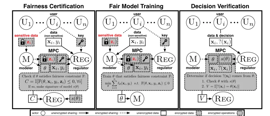
1. Fairness certification. Given a model and a dataset of individuals, check that the model satisfies a given fairness constraint (we consider several notions from the literature, see Section2.2); if yes, generate a certificate.

2. Fair model training. Given a dataset of individuals, learn a model guaranteed and certified to be fair. 3. Decision verification. A malicious modeler might go

through fair model training, but then use a different model in practice. To address such accountability concerns (Kroll et al.,2016), we efficiently provide for an indi-vidual to challenge a received outcome, verifying that it matches the outcome from the previously certified model.

We rely on recent theoretical developments in MPC (see Section3) which we extend to admit linear constraints in order to enforce fairness requirements. These extensions may be of independent interest. We demonstrate the real-world efficacy of our methods, and shall make our code publicly available.

2. Fairness and Privacy Requirements

Here we formalize our setup and requirements.

2.1. Assumptions and Incentives

We assume three categories of participants: amodelerM,

aregulatorREG, andusersU1, . . . ,Un. For each user, we consider a vector of sensitive features (or attributes, we use the terms interchangeably)zi ∈ Z (e.g., ethnicity or gender) which might be a source of discrimination, and a vector of non-sensitive featuresxi ∈ X (discrete or real). Additionally, each user has a non-sensitive featureyi∈ Y which the modeler M would like to predict—thelabel(e.g.,

loan default). In line with current work in fair learning, we

assume that allziandyiattributes are binary, though our MPC approach could be extended to multi-label settings. The source of societal concern is that sensitive attributeszi are potentially correlated withxioryi.

Modeler M wishes to train a modelfθ : X → Y, which accurately maps features xi to labelsyi, in a supervised fashion. We assume M needs to keep the model private for intellectual property or other business reasons. The model

fθdoes not use sensitive informationzias input to prevent disparate treatment (direct discrimination).

For each user Ui, M observes or is provided xi, yi. The sensitive information inziis required to ensurefθmeets a given disparate impact fairness conditionF(see Section2.2). While each user Uiwantsfθto meetF, they also wish to keepziprivate from all other parties. The regulator REG aims to ensure that M deploys only models that meet fair-ness conditionF. It has no incentive to collude with M (if collusion were a concern, more sophisticated cryptographic protocols would be required). Further, the modeler M might be legally obliged to demonstrate to the regulator REGthat

their model meets fairness conditionFbefore it can be pub-licly deployed. As part of this, REGalso has a positive duty

to enable the training of fair models.

In Section 2.3, we define and address three fundamental problems in our setup: certification, training, and verifica-tion. For each problem, we present its functional goal and its privacy requirements. We refer toD=_{(xi, yi)}ni=1and Z=_{zi}ni=1as the non-sensitive and sensitive data, respec-tively. In Section2.2, we first provide necessary background on various notions of fairness that have been explored in the fair learning literature.

2.2. Fairness Criteria

In large part, works that formalize fairness in machine learn-ing do so by balanclearn-ing a certain condition between groups of people with different sensitive attributes, z versusz0_. Several possible conditions have been proposed. Popular choices include (wherey∈ {0,1}andyˆis the prediction of a machine learning model):

P(ˆy=y_|z) =P(ˆy=y_|z0) (acc) (1)

P(ˆy=y_|z, y= 1) =P(ˆy=y_|z0_{, y= 1) (TPR) (2)}

P(ˆy=y_|z, y= 0) =P(ˆy=y_|z0, y= 0) (TNR) (3)

P(ˆy=y_|z,yˆ= 1) =P(ˆy=y_|z0_{,yˆ= 1) (PPV) (4)}

P(ˆy=y|z,yˆ= 0) =P(ˆy=y|z0,yˆ= 0) (NPV) (5)

In this work we focus on a variant of eq. (6), formulated as a constrained optimization problem byZafar et al.(2017c) mimicking thep%-rule (Biddle,2006): for any binary pro-tected attributez_{∈ {}0,1_}, it aims to achieve

min

_{P(ˆy= 1}

|z= 1)

P(ˆy= 1_|z= 0),

P(ˆy= 1|z= 0)

P(ˆy= 1_|z= 1)

≥₁₀₀p . (7)

We believe that in future work, a similar MPC approach could also be used for conditions (1), (2) or (3)—i.e., all the other measures which, to our knowledge, have been addressed with efficient standard (non-private) methods.

2.3. Certification, Training, and Verification

Fairness certification. Given a notion of fairnessF, the modeler M would like to work with the regulator REGto obtain a certificate that model fθ is fair. To do so, we propose that users send their non-sensitive dataDto REG;

and sendencryptedversions of their sensitive dataZto both M and REG. Neither M nor REGcan read the sensitive data.

However, we can design a secure protocol between M and REG(described in Section3) to certify if the model is fair.

This setup is shown in Figure1(Left).

While both REG and M learn the outcome of the

certifi-cation, we require the followingprivacy constraints: (C1) privacy of sensitive user data: no one other than Ui ever learnsziin the clear, (C2)model secrecy:only M learnsfθ in the clear, and (C3)minimal disclosure ofDtoREG:only

REGlearnsDin the clear.

Fair model training. How can a modeler M learn a fair model without access to users’ sensitive dataZ? We propose to solve this by having users send their non-sensitive data Dto M and to distribute encryptions of their sensitive data to M and REGas in certification. We shall describe a secure MPC protocol between M and REGto train a fair modelfθ privately. This setup is shown in Figure1(Center).

Privacy constraints: (C1) privacy of sensitive user data, (C2)

model secrecy, and (C3) minimal disclosure ofDto M.

Decision verification. Assume that a malicious M has had modelfθ successfully certified by REGas above. It then swapsfθfor another potentially unfair modelfθ0 in the real world. When a user receives a decisionyˆ, e.g., her mortgage is denied, she can then challenge that decision by asking REGfor a verificationV. The verification involves

M and REG, and consists of verifying thatfθ0(x) =fθ(x), wherexis the user’s non-sensitive data. This ensures that the user would have been subject to the same result with the certified modelfθ, even iffθ0 6=fθandfθ0 is not fair. Hence, while there is no simple technical way to prevent a malicious M from deploying an unfair model, it will get

caught if a user challenges a decision that would differ underfθ. This setup is shown in Figure1(Right).

Privacy constraint: While REGand the user learn the out-come of the verification, we require (C1) privacy of sensitive user data, and (C2) model secrecy.

2.4. Design Choices

We use a regulator for several reasons. Given fair learning is of most benefit to vulnerable individuals, we do not wish to deter adoption with high individual burdens. While MPC could be carried out without the involvement of a regulator, using all users as parties, this comes at a significantly greater computational cost. With current methods, taking that ap-proach would be unrealistic given the size of the user-base in many domains of concern, and would furthermore require all users to be online simultaneously. Introducing a regula-tor removes these barriers and leaves users’ computational burden at a minimum level, with envisaged applications practical with only their web browsers.

In cases where users are uncomfortable sharing D with either REGor M, it is trivial to extend all three tasks such

that all of xi, yi,zi remain private throughout, with the computation cost increasing only by a factor of 2. This extension would sometimes be desirable as it restricts the view of M to the final model, prohibiting inferences aboutZ whenDis known. However, this setup hinders exploratory data analysis by the modeler which might promote robust model-building, and, in the case of verification, validation by the regulator that user-provided data is correct.

3. Our Solution

Our proposed solution to these three problems is to use Multi-Party Computation (MPC). Before we describe how it can be applied to fair learning, we first present the basic principles of MPC, as well as its limitations particularly in the context of machine learning applications.

3.1. MPC for Machine Learning

Multi-Party Computation protocols allow two partiesP1 andP2holding secret valuesx1andx2to evaluate an agreed-upon function f, viay = f(x1, x2)in a way in which the parties (either both or one of them) learnonlyy. For example, iff(x1, x2) =I(x1< x2), then the parties would learn which of their values is bigger, but nothing else.1_This corresponds to the well-knownYao’s millionaires problem:

two millionaires want to conclude who is richer without disclosing their wealth to each other. The problem was introduced by Andrew Yao in 1982, and kicked off the area of multi-party computation in cryptography.

Reg

Fairness Certification

modeler

user

regulator

Reg

sensitive data

M

U

U

U

Fair Model Training

data

(non-sensitive) key

Decision Verification

✓

(zi)

xi, yi

Check if✓satisfies fairness constraintF:

Reg

MPC

If so, make signature of models(✓)

C=I[F(✓,xi, yi,zi)0,8i]

C

xi, yi (zi)

s(✓)

modeler regulator

Reg

sensitive data

M

U

U1

U

data

(non-sensitive) key

✓

(zi)

xi, yi MPC xi, yi (zi)

min

✓ n

X

i=1

`✓(xi, yi)s.t.F(✓,xi, yi,zi)0

Train✓that satisfies fairness constraintF:

M

✓

modeler regulator

Reg

M

U

U1

U

✓

MPC s(✓)

data & decision

xi,?(xi)

Determine if decision ?(xi) comes from✓: xi,?(xi)

1. Check✓withs(✓) 2.V=I[?(xi) =✓(xi)]

V

user user

unencrypted sharing: encrypted sharing: encrypted data:

actor: unencrypted data: encrypted operations:

Figure 1.Our setup forFairness certification(Left),Fair model training(Center), andDecision verification(Right).

In our setting—instead of a simple comparison as in the millionaires problem—f will be either (i) a procedure to check the fairness of a model and certify it, (ii) a machine learning training procedure with fairness constraints, or (iii) a model evaluation to verify a decision. The two parties involved in our computation are the modeler M and the regulator REG. The inputs depend on the case (see Figure1).

As generic solutions do not yet scale to real-world data anal-ysis tasks, one typically has to tailor custom protocols to the desired functionality. This approach has been followed successfully for a variety of machine learning tasks such as logistic and linear regression (Nikolaenko et al.,2013b;

Gasc´on et al.,2017;Mohassel & Zhang,2017), neural net-work training (Mohassel & Zhang,2017) and evaluation (Juvekar et al.,2018; Liu et al.,2017), matrix factoriza-tion (Nikolaenko et al.,2013a), and principal component analysis (Al-Rubaie et al.,2017). In the next section we review challenges beyond scalability issues that arise when implementing machine learning algorithms in MPC.

3.2. Challenges in Multi-Party Machine Learning

MPC protocols can be classified into two groups depend-ing on whether the target function is represented as either a Boolean or arithmetic circuit. All protocols proceed by having the parties jointly evaluate the circuit, processing it gate by gate while keeping intermediate values hidden from both parties by means of a secret sharing scheme. While rep-resenting functions as circuits can be done without losing expressiveness, it means certain operations are impracti-cal. In particular, algorithms that execute different branches depending on the input data will explode in size when im-plemented as circuits, and in some cases lose their run time guarantees (e.g., consider binary search).

Crucially, this applies tofloating-point arithmetic. While

this is work in progress, state-of-the-art MPC floating-point arithmetic implementations take more than15milliseconds to multiply two 64bit numbers (Demmler et al.,2015a, Table 4), which is prohibitive for our applications. Hence, machine learning MPC protocols are limited tofixed-point

arithmetic. Overcoming this limitation is a key challenge for the field. Another necessity for the feasibility of MPC is to approximate non-linear functions such as the sigmoid, ideally by (piecewise) linear functions.

3.3. Our MPC Protocols

Input sharing. To implement the functionality from Fig-ure 1, we first need a secure procedure for the users to

secret sharea sensitive value, for example her race, with the

modeler M and the regulator REG. We useadditive secret sharing. A valuezis represented in a finite domainZq—we useq= 264_{. To sharez, the user samples a valuerfromZ}

q uniformly at random, and sendsz₋rto M andrto REG. Whilezcan be reconstructed (and subsequently operated

on) inside the MPC computation by means of a simple addi-tion, each share on its own does not reveal anythingz(other

than that it is inZq). One can think of arithmetic sharing as a “distributed one-time pad”.

In Figure1, we now reinterpret the key held by REGand

the encrypted z by M, as their corresponding shares of

the sensitive attributes and denote them byhzi1andhzi2 respectively. The idea of privately outsourcing computation to two non-colluding parties in this way is recurrent in MPC, and often referred to as the two-server model (Mohassel & Zhang,2017;Gasc´on et al.,2017;Nikolaenko et al.,2013b;

Al-Rubaie et al.,2017).

Signing and checking a model. Note thatcertification

constraintF, and repeatedly evaluate partial models on the training dataset (using gradient descent). Hence, certifica-tionandverificationdo not add technical difficulties over

training, which is described in detail in Section4. However, for verification, we still need to “sign” the model, i.e., REG

should obtain a signatures(θ)as a result of model certifi-cation, see Figure1(Left). This signature is used to check

in the verification phase, whether a given modelθ0from M

satisfiess(θ0) =s(θ)for a certified fair modelθ(in which

caseθ=θ0with high probability). Moreover, we need to

preserve the secrecy of the model, i.e., REGshould not be

able to recoverθfroms(θ). These properties, given that

the space of models is large, calls for a cryptographic hash function, such as SHA-256.

Additionally, in our functionality, the hash of θ should

be computed inside MPC, to hide θ from REG. Fortu-nately, cryptographic hashes such as SHA-256 are a com-mon benchmark functionality in MPC, and their execution is highly optimized. More concretely, the overhead of com-putings(θ), which needs to be done both for certification

and verification is of the order of fractions of a second (Keller et al.,2013, Figure 14). While cryptographic hash functions have various applications in MPC, we believe the application to machine learning model certification is novel. Hence, certification is implemented in MPC as a check that

θsatisfies the criterionF, followed by the computation of s(θ). On the other hand, for verification, the MPC protocol

first computes the signature of the model provided by M, and then proceeds with a prediction as long as the computed signature matches the one obtained by REGin the verifi-cation phase. An alternative solution is possible based on symmetric encryption under a shared key, as highly efficient MPC implementations of block ciphers such as AES are available (Keller et al.,2017).

Fair training. To realize the fair trainingfunctionality

from the previous section, we follow closely the techniques recently introduced byMohassel & Zhang(2017). Specif-ically, we extend their custom MPC protocol for logistic regression to additionally handle linear constraints. This ex-tension may be of independent interest, and has applications for privacy-preserving machine learning beyond fairness. The concrete technical difficulties in achieving this goal, and how to overcome them, are presented in the next sec-tion. The formal privacy guarantees of our fair training protocol are stated in the following proposition.

Proposition 1. For non-colludingMandREG, our protocol implements the fair model training functionality satisfying constraints (C1)-(C3) in Section2.3in the presence of a semi-honest adversary.

The proof holds in the random oracle model, as a standard simulation argument combining several MPC primitives

(Mohassel & Zhang,2017;Gasc´on et al.,2017). It lever-ages security of arithmetic sharing, garbled circuits, and oblivious transfer protocols in the semi-honest model ( Gol-dreich et al.,1987). A general introduction to MPC, as well as a description of the relevant techniques from ( Mohas-sel & Zhang,2017) used in our protocol, can be found in SectionAin the appendix.

4. Technical Challenges of Fair Training

We now present our tailored approaches for learning and evaluating fair models with encrypted sensitive attributes. We do this via the following contributions:

• We argue that current optimization techniques for fair learning algorithms are unstable for fixed-point data, which is required by our MPC techniques.

• We describe optimization schemes that are well-suited for learning over fixed-point number representations. • We combine tricks to approximate non-linear functions

with specialized operations to make fixed-point arithmetic feasible and avoid over- and under-flows.

The optimization problem at hand is to learn a classifierθ

subject to a (often convex) fairness constraintF(θ):

min θ

n

X

i=1

`θ(xi, yi) subject to F(θ)≤0, (8)

where `θ is a loss term (the logistic loss in this work). We collect user data from U1, . . . ,Uninto matricesX∈ Rn×d_{,Z∈ {0,1}}n×p_{and a label vectory∈ {0,1}}n_.

Zafar et al.(2017c) use a convex approximation of thep

%-rule, see eq. (7), for linear classifiers to derive the constraint:

F(θ) = 1

n|Zˆ

>_Xθ

| −c, (9)

where_Zˆ _{is the matrix of all ˆzi := zi −¯zand c ∈ R}d is a constant vector corresponding to the tightness of the fairness constraint. Here,¯zis the mean of all inputszi. With A:=1_/nZˆ>X, the_p%constraintreadsF_{(θ) =|Aθ| −}c, where the absolute value is taken element-wise.

4.1. Current Techniques

To solve the optimization problem in eq. (8), with the fair-ness function_Fin eq. (9),Zafar et al.(2017c) use Sequen-tial Least Squares Programming (SLSQP). This technique works by reformulating eq. (8) as a sequence of Quadratic Programs (QPs). After solving each QP, their algorithm uses the Han-Powell method, a quasi-Newton method that itera-tively approximates the HessianHof the objective function via the update

Ht+1=Ht+ l∆l>∆

θ>_∆l∆ −

Htθ∆θ>∆Ht

θ>_∆Htθ∆

where l∆ = l(θt+1,λt+1)−l(θt,λt) and l(θt,λt) =

Pn

i=1`θt(xi, yi) +λ >

F(θt)is the Lagrangian of eq. (8). Finally,θ∆=θt+1−θt.

There are two issues with this approach from an MPC per-spective. First, solving a sequence of QPs is prohibitively time-consuming in MPC. Second, while the above Han-Powell update performs well on floating-point data, the two divisions by non-constant, non-integer numbers easily underflow or overflow with fixed-point numbers.

4.2. Fixed-Point-Friendly Optimization Techniques

Instead, to solve the optimization problem in eq. (8), we perform stochastic gradient descent and experiment with the following techniques to incorporate the constraints.

Lagrangian multipliers.Here we minimize

L:= 1

n

n

X

i=1

`BCEθ (xi, yi) +λ

>_max{F(θ),0 },

using stochastic gradient descent, i.e., alternating updates

θ _← θ ₋ηθ∇θL and λ ← max{λ + ηλ∇λL,0}, whereηθ, ηλare the learning rates.

Projected gradient descent.For this method, consider

specif-ically thep%-rule based notionF(θ) =|Aθ_{| −}c. We first

define _Aˆ _{as the matrix consisting of the rows of A for} whichF(θ)>0, i.e., where the constraint is active. In each step, we project the computed gradient of the binary-cross-entropy loss_LBCE_{—either of a single example or averaged} over a minibatch—back into the constraint set, i.e.,

θ_←θ₋ηθ(Idd−Aˆ>( ˆAAˆ>)−1A)ˆ ∇θ`BCEθ . (10)

Interior point log barrier (Boyd & Vandenberghe,2004).

We can approximate eq. (8) for the p%-rule

con-straintF(θ) =|Aθ_|−cby: minimizePni=1`BCEθ (xi, yi)−

1 t

Pp

j=1 log(a>jθ+cj) + log(−a>jθ+cj), whereajis thejth row ofA. The parameterttrades off the approx-imation of the true objective (I−(u) = 0foru ≤ 0and

I−(u) =∞foru >0) and the smoothness of the objective function. Throughout trainingtis increased, allowing the solution to move closer to the boundary. As the gradient of the objective has a simple closed form representation, we can perform regular (stochastic) gradient descent.

After extensive experiments (see Section5) we found the La-grangian multipliers technique to work best, both in yielding high accuracies, reliably staying within the constraints and being robust to hyperparameter changes such as learning rates or the batch size. For a proof of concept, in Section5

we focus on thep%-rule, i.e., eq. (9). Note that the gradients

for eq. (2) and eq. (3) take a similarly simple form, i.e., bal-ancing the true positive or true negative rates (corresponding to equal opportunity or equal odds) is simple to implement

for the Lagrangian multiplier technique, but harder for pro-jected gradient descent. However, these fairness notions are more expensive as we have to computeZ>_{Xfor each} update step, instead of pre-computing it once at the begin-ning of traibegin-ning, see Algorithm1in the appendix. We could speed up the computation again by evaluating the constraint only on the current minibatch for each update, in which case we risk violating the fairness constraint.

MPC-friendliness. For eq. (9), we can compute the gra-dient updates in all three methods with elementary linear algebra operations (matrix multiplications) and a single eval-uation of the logistic function. While MPC is well suited for linear operations, most nonlinear functions are prohibitively expensive to evaluate in an MPC framework. Hence we tried two piecewise linear approximations forσ(x). The

first was recently suggested for machine learning in an MPC context (Mohassel & Zhang, 2017) and is simply constant0and1forx <−0.5andx >0.5respectively, and linear in between. The second uses the optimal first order Chebychev polynomial on each interval[x, x+ 1] forx ∈ {−5,−4, . . . ,4}, and is constant0 or1 outside of[₋5,5](Faiedh et al.,2001). While it is more accurate, we only report results for the simpler first approximation, as it yielded equal or better results in all our experiments. As the largest number that can be represented in fixed-point format withminteger andmfractional bits is roughly2m₊ 1, overflow becomes a common problem. Since we whiten the featuresXcolumn-wise, we need to be careful whenever we add roughly2m_{numbers or more, because we cannot} even represent numbers greater than2m_{. In particular, the} minibatch size has to be smaller than this limit. For largen,

the multiplicationZ>_{Xin the fairness functionFfor the}

p%-rule is particularly problematic.

Hence, we split both factors into blocks of size b ×b

with b < 2m _{and normalize the result of each blocked} matrix multiplication bybbefore adding up the blocks. We then multiply the sum byb_{/n > 2}−m. As long as _b, b_/n (and thus alson_/b) can be represented with sufficient preci-sion, which is the case in all our experiments, this procedure avoids under- and overflow. Note that we require the sam-ple size nto be a multiple ofb. In practice, we have to

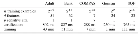
Table 1.Dataset sizes and online timing results of MPC certifica-tion and training over 10 epochs with batch size 64.

Adult Bank COMPAS German SQF

ntraining examples 214 ₂15 ₂12 ₂9 ₂16

dfeatures 51 62 7 24 23

psensitive attr. 1 1 7 1 1

certification 802 ms 827 ms 288 ms 250 ms 765 ms training 43 min 51 min 7 min 1 min 111 min

Algorithm1in Section B in the appendix describes the computations M and REGhave to run for fair model training using the Lagrangian multiplier technique and thep%-rule from eq. (9). We implicitly assume all computations are performed jointly on additively shared secrets.

5. Experiments

The root cause for most technical difficulties pointed out in the previous section is the necessity to work with fixed-point numbers and the high computational cost of MPC. Hence, major concerns are loss of precision and infeasible running times. In this section, we show how to overcome both doubts and that fair training, certification and verification are feasible for realistic datasets.

5.1. Experimental Setup and Datasets

We work with two separate code bases. Our Python code does not implement MPC, to be able to flexibly switch between floating and fixed-point numbers as well as exact non-linear functions and their approximations. We use it mostly for validation and empirical guidance in our design choices. The full MPC protocol is implemented in C++ on top of the Obliv-C garbled circuits framework (Zahur & Evans,2015a) and the Absentminded Crypto Kit (lib). This is done as described in Section3for the Lagrangian multiplier technique (see SectionAin the appendix for more details). It accurately mirrors the computations performed by the first implementation on encrypted data.2_{Except for} the timing results in Table1, all comparisons with floating-point numbers or non-linearities were done with the versatile Python implementation. Details about parameters and the algorithm can be found in SectionBin the appendix. We consider 5 real world datasets, namely the adult (Adult),

German credit (German), and bank market (Bank) datasets

from the UCI machine learning repository (Lichman,2013), the stop, question and frisk 2012 dataset (SQF),3and the

COMPAS dataset (Angwin et al.,2016) (COMPAS). For

practical purposes (see Section 4), we subsample2i ex-amples from each dataset with the largest possiblei, see

Table1. Moreover, we also run on synthetic data, generated

2_{Code is available at https://github.com/}

nikikilbertus/blind-justice

3_{https://perma.cc/6CSM-N7AQ}

as described byZafar et al.(2017c, Section 4.1), as it allows us to control the correlation between the sensitive attributes and the class labels. It is thus well suited to observe how dif-ferent optimization techniques handle the fairness-accuracy trade off. For comparison we use the SLSQP approach described in Section4.1as a baseline. We run all meth-ods for a range of constraint values in[10−4_,100_{]and a} corresponding range for SLSQP.

In the plots in this section, discontinuations of lines indicate failed experiments. The most common reasons are overflow and underflow for fixed-point numbers, and instability due to exploding gradients. Plots and analyses for the remaining datasets can be found in SectionCin the appendix.

5.2. Comparing Optimization Techniques

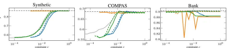
First we evaluate which of the three optimization techniques works best in practice. Figure2shows the test set accuracy over the constraint value. By design, the synthetic dataset exhibits a clear trade-off between accuracy and fairness. The

Lagrangetechnique closely follows the (dotted) baseline from (Zafar et al.,2017c), whereasiplbperforms slightly worse (and fails for smallc). Even though theprojected

gradient method formally satisfies the proxy constraint for thep%rule, it does so by merely shrinking the parameter vectorθ, which is why it also fails for smallc. We analyze

this behavior in more detail in SectionCin the appendix. The COMPAS dataset is the most challenging as it contains 7 sensitive attributes, one of which has only 10 positive instances in the training set. Since we enforce the fairness constraint individually for each sensitive attribute (we ran-domly picked one for visualization), the classifier tends to collapse to negative predictions. All three methods maintain close to optimal accuracy in the unconstrained region, but collapse more quickly than SLSQP. This example shows that thep%-rule proxy itself needs careful interpretation when

applied to multiple sensitive attributes simultaneously and that our SGD based approach seems particularly prone to collapse in such a scenario. On the Bank dataset accuracy in-creases foriplbandLagrangewhen the constraint becomes active ascdecreases until they match the baseline.

Deter-mining the cause of this—perhaps unintuitive—behavior requires further investigation. We currently suspect the con-straint to act as a regularizer. Theprojectedgradient method is unreliable on the Bank dataset.

Empirically, the Lagrangian multiplier technique is most robust with maximal deviations of accuracy from SLSQP of<4% across the 6 datasets and all constraint values. We

10−4 ₁₀−2 ₁₀0

0.6 0.7 0.8

constraintc

accurac

y

Synthetic

10−4 ₁₀−2 ₁₀0

0.55 0.6 0.65 0.7

constraintc

COMPAS

10−4 ₁₀−2 ₁₀0

0.8 0.82 0.84 0.86 0.88 0.9

constraintc

Bank

Figure 2.Test set accuracy over thep%value for different optimization methods (blue: iplb,orange: projected,green: Lagrange) and

either no approximation (continuous) or a piecewise linear approximation (dashed) of the sigmoid using floating-point numbers. The gray

dotted line is the baseline (see Section4.1) and the black dashed line is unconstrained logistic regression (from scikit-learn).

10−4 ₁₀−2 ₁₀0

0.2 0.4 0.6 0.8

constraintc

fraction

with

ˆ

y

=

1 Synthetic

10−4 ₁₀−2 ₁₀0

0 0.2 0.4

constraintc

COMPAS

10−4 ₁₀−2 ₁₀0

0 0.2 0.4 0.6

constraintc

Bank

Figure 3.The fraction of people withz= 0(continuous/dotted) andz= 1(dashed/dash-dotted) who get assigned positive outcomes

(red: no approx. + float,purple: no approx. + fixed,yellow: pw linear + float,turquoise: pw linear + fixed, gray: baseline).

5.3. Fair Training, Certification and Verification

Figure3shows how the fractions of users with positive out-comes in the two groups (z= 0is continuous andz= 1is dashed) are gradually balanced as we decrease the fairness constraintc. These plots can be interpreted as the degree

to which disparate impact is mitigated as the constraint is tightened. The effect is most pronounced for the synthetic dataset by construction. As discussed above, the collapse for the COMPAS dataset occurs faster than for SLSQP due to the constraints from multiple sensitive attributes. In the Bank dataset, for largec—before the constraint becomes active—the fractions of positive outcomes forz = 1 dif-fer, which is related to the slightly suboptimal accuracy at largec that needs further investigation. However, as the

constraint becomes active, the fractions are balanced at a similar rate as the baseline. Overall, our Lagrangian mul-tiplier technique with fixed point numbers and piecewise linear approximations of non-linearities robustly manages to satisfy the p%-rule proxy at similar rates as the baseline with only minor losses in accuracy on all but the challenging COMPAS dataset.

In Table1we show the online running times of 10 training epochs on a laptop computer. While training takes several orders of magnitudes longer than a non-MPC implementa-tion, our approach still remains feasible and realistic. We use the one time offline precomputation of multiplication triples described and timed inMohassel & Zhang(2017, Table 2). As pointed out in Section3, certification of a trained model requires checking whetherF(θ) > 0. We

already perform this check at least once for each gradient

update during training. It only takes a negligible fraction of the computation time, see Table1. Similarly, the operations required for certification stay well below one second.

Discussion.In this section, we have demonstrated the prac-ticability of private and fair model training, certification and verification using MPC as described in Figure1. Using the methods and tricks introduced in Section4, we can over-come accuracy as well as over- and underflow concerns due to fixed-point numbers. Offline precomputation combined with a fast C++ implementation yield viable running times for reasonably large datasets on a laptop computer.

6. Conclusion

Acknowledgments

The authors would like to thank Chris Russell and Phillipp Schoppmann for useful discussions and help with the imple-mentation, as well as the anonymous reviewers for helpful comments. AG and MK were supported by The Alan Turing Institute under the EPSRC grant EP/N510129/1. MV was supported by EPSRC grant EP/M507970/1. AW acknowl-edges support from the David MacKay Newton research fellowship at Darwin College, The Alan Turing Institute under EPSRC grant EP/N510129/1 & TU/B/000074, and the Leverhulme Trust via the CFI.

References

Absentminded crypto kit. https://bitbucket.org/ jackdoerner/absentminded-crypto-kit.

Al-Rubaie, M., Wu, P. Y., Chang, J. M., and Kung, S. Privacy-preserving PCA on horizontally-partitioned data. InDSC, pp. 280–287. IEEE, 2017.

Angwin, J., Larson, J., Mattu, S., and Kirchner, L. Ma-chine bias: There is software used across the country to predict future criminals. and it is biased against blacks.

ProPublica, May, 23, 2016.

Barocas, S. and Selbst, A. D. Big data’s disparate impact.

California Law Review, 104:671–732, 2016.

Bennett Capers, I. Blind justice. Yale Journal of Law & Humanities, 24:179, 2012.

Biddle, D. Adverse impact and test validation: A practi-tioner’s guide to valid and defensible employment testing.

Gower Publishing, Ltd., 2006.

Boyd, S. and Vandenberghe, L.Convex optimization.

Cam-bridge university press, 2004.

Calders, T. and ˇZliobait˙e, I. Why unbiased computational processes can lead to discriminative decision procedures. InDiscrimination and Privacy in the Information Society,

pp. 43–59. Springer, 2012.

Damg˚ard, I., Pastro, V., Smart, N. P., and Zakarias, S. Mul-tiparty computation from somewhat homomorphic en-cryption. InCRYPTO, volume 7417 ofLecture Notes in Computer Science, pp. 643–662. Springer, 2012.

Demmler, D., Dessouky, G., Koushanfar, F., Sadeghi, A., Schneider, T., and Zeitouni, S. Automated synthesis of optimized circuits for secure computation. InACM Conference on Computer and Communications Security,

pp. 1504–1517. ACM, 2015a.

Demmler, D., Schneider, T., and Zohner, M. ABY – a framework for efficient mixed-protocol secure two-party computation. InNDSS. The Internet Society, 2015b.

Dwork, C., Hardt, M., Pitassi, T., Reingold, O., and Zemel, R. Fairness through awareness. InProceedings of the 3rd Innovations in Theoretical Computer Science Conference,

ITCS ’12, pp. 214–226. ACM, 2012.

Faiedh, H., Gafsi, Z., and Besbes, K. Digital hardware implementation of sigmoid function and its derivative for artificial neural networks. Proceeding of the 13th International Conference on Microelectronics, 2001., pp.

189 – 192, 11 2001.

Feldman, M., Friedler, S., Moeller, J., Scheidegger, C., and Venkatasubramanian, S. Certifying and removing dis-parate impact. InProceedings of the 21th ACM SIGKDD International Conference on Knowledge Discovery and Data Mining, pp. 259–268, 2015.

Fredrikson, M., Jha, S., and Ristenpart, T. Model inver-sion attacks that exploit confidence information and ba-sic countermeasures. InProceedings of the 22nd ACM SIGSAC Conference on Computer and Communications Security, pp. 1322–1333, 2015.

Friedler, S. A., Scheidegger, C., and Venkatasubrama-nian, S. On the (im)possibility of fairness. 2016. arXiv:1609.07236v1 [cs.CY].

Gasc´on, A., Schoppmann, P., Balle, B., Raykova, M., Do-erner, J., Zahur, S., and Evans, D. Privacy-Preserving Distributed Linear Regression on High-Dimensional Data.

Proceedings on Privacy Enhancing Technologies, 2017

(4):345–364, October 2017.

Goldreich, O.The Foundations of Cryptography – Volume 2, Basic Applications. Cambridge University Press, 2004.

Goldreich, O., Micali, S., and Wigderson, A. How to play any mental game or A completeness theorem for proto-cols with honest majority. InSTOC, pp. 218–229. ACM,

1987.

Graham, C. NHS cyber attack: Everything you need to know about ’biggest ransomware’ offensive in history.

Telegraph, May 20, 2017.

Grgi´c-Hlaˇca, N., Zafar, M. B., Gummadi, K. P., and Weller, A. Beyond distributive fairness in algorithmic decision making: Feature selection for procedurally fair learning. InAAAI, 2018.

Handel, P., Skog, I., Wahlstrom, J., Bonawiede, F., Welch, R., Ohlsson, J., and Ohlsson, M. Insurance telematics: Opportunities and challenges with the smartphone solu-tion.IEEE Intelligent Transportation Systems Magazine,

6(4):57–70, 2014.

Juvekar, C., Vaikuntanathan, V., and Chandrakasan, A. Gazelle: A Low Latency Framework for Secure Neu-ral Network Inference. IACR Cryptology ePrint Archive,

2018:73, 2018.

Keller, M., Scholl, P., and Smart, N. P. An architecture for practical actively secure MPC with dishonest majority. InACM Conference on Computer and Communications Security, pp. 549–560. ACM, 2013.

Keller, M., Orsini, E., Rotaru, D., Scholl, P., Soria-Vazquez, E., and Vivek, S. Faster secure multi-party computation of AES and DES using lookup tables. InACNS, volume

10355 ofLecture Notes in Computer Science, pp. 229–

249. Springer, 2017.

Keller, M., Pastro, V., and Rotaru, D. Overdrive: Mak-ing SPDZ great again. In EUROCRYPT (3), volume

10822 ofLecture Notes in Computer Science, pp. 158–

189. Springer, 2018.

Kroll, J. A., Huey, J., Barocas, S., Felten, E. W., Reiden-berg, J. R., Robinson, D. G., and Yu, H. Accountable algorithms.University of Pennsylvania Law Review, 165,

2016.

Lichman, M. UCI machine learning repository, 2013. URL http://archive.ics.uci.edu/ml.

Lindell, Y. How To Simulate It – A Tutorial on the Simula-tion Proof Technique.IACR Cryptology ePrint Archive,

2016:46, 2016.

Liu, J., Juuti, M., Lu, Y., and Asokan, N. Oblivious neural network predictions via minionn transformations. InCCS,

pp. 619–631. ACM, 2017.

Mohassel, P. and Zhang, Y. SecureML: A system for scal-able privacy-preserving machine learning. InIEEE Sym-posium on Security and Privacy (SP), pp. 19–38, 2017.

Nikolaenko, V., Ioannidis, S., Weinsberg, U., Joye, M., Taft, N., and Boneh, D. Privacy-preserving matrix factoriza-tion. InACM Conference on Computer and Communica-tions Security, pp. 801–812. ACM, 2013a.

Nikolaenko, V., Weinsberg, U., Ioannidis, S., Joye, M., Boneh, D., and Taft, N. Privacy-preserving ridge re-gression on hundreds of millions of records. InIEEE Symposium on Security and Privacy, pp. 334–348. IEEE

Computer Society, 2013b.

Schreurs, W., Hildebrandt, M., Kindt, E., and Vanfleteren, M.Cogitas, Ergo Sum. The Role of Data Protection Law

and Non-discrimination Law in Group Profiling in the Private Sector. InProfiling the European Citizen, pp.

241–270. Springer, 2008.

Tram`er, F., Zhang, F., Juels, A., Reiter, M. K., and Risten-part, T. Stealing machine learning models via prediction apis. InUSENIX Security Symposium, pp. 601–618, 2016.

Veale, M. and Binns, R. Fairer machine learning in the real world: Mitigating discrimination without collecting sensitive data. Big Data & Society, 4(2), 2017.

Veale, M. and Edwards, L. Clarity, Surprises, and Further Questions in the Article 29 Working Party Draft Guidance on Automated Decision-Making and Profiling. Computer Law & Security Review, 2018. doi: 10.1016/j.clsr.2017.

12.002.

Yao, A. C.-C. How to Generate and Exchange Secrets (Ex-tended Abstract). InFOCS, pp. 162–167. IEEE Computer

Society, 1986.

Zafar, M. B., Valera, I., Gomez-Rodriguez, M., and Gum-madi, K. P. Fairness beyond disparate treatment & dis-parate impact: Learning classification without disdis-parate mistreatment. InWWW, 2017a.

Zafar, M. B., Valera, I., Rodriguez, M., Gummadi, K., and Weller, A. From parity to preference-based notions of fair-ness in classification. InAdvances in Neural Information Processing Systems, pp. 228–238, 2017b.

Zafar, M. B., Valera, I., Rodriguez, M. G., and Gummadi, K. P. Fairness Constraints: Mechanisms for Fair Classifi-cation. InAISTATS, 2017c.

Zahur, S. and Evans, D. Obliv-c: A language for extensible data-oblivious computation. IACR Cryptology ePrint Archive, 2015:1153, 2015a.

Zahur, S. and Evans, D. Obliv-C: A Language for Extensible Data-Oblivious Computation. IACR Cryptology ePrint Archive, 2015:1153, 2015b.

ˇZliobait˙e, I. and Custers, B. Using sensitive personal data may be necessary for avoiding discrimination in data-driven decision models.Artificial Intelligence and Law,

A. Details of the MPC Protocols

Secret sharing. A secret sharing scheme allows one to split a valuex(the secret) among two parties, so that no party has unilateral access tox. In our setting, a user Alice will secret share a sensitive value, for example her race, among a modeler M and a regulator REG. Several secret sharing schemes exist, includingShamir secret sharing,xor sharing,Yao sharing, orarithmetic multiplicative/additive sharing. In this work we alternate between Yao sharing and

additive sharing for efficiency. In the latter, the valuexis

represented in a finite domainZqwith, for exampleq= 232. To share her race, Alice samples a valuerfromZquniformly at random, and sendsx−rto M andrto REG. We call each

ofx−randrashare, and denote them as_hxi1andhxi2. Now M and REGcan recoverxby adding their shares, but

each share on its own does not reveal anything about the value ofx(other than that it is smaller thanq). Note that the case whereq= 2corresponds to xor sharing.

Function evaluation. MPC can be classified in two groups depending on how f is represented: either as a

Boolean or arithmetic circuit. All protocols proceed by having the parties jointly evaluate the circuit, processing it gate by gate. For each gategfor which the value for the

input wiresx, yis shared among the parties, the parties run

a subprotocol to produce the valuez=g(x, y)of the output wire, again shared, without revealing any information in the process. In the setting where we use arithmetic additive sharing, the two parties M and REGhold shares,hx_i1,hyi1 andhx_i2,hyi2, respectively. In this case,f is represented as an arithmetic circuit, and hence each gategin the circuit is either an addition or a multiplication. Note that ifgis an

addition gate, then a sharing ofz=g(x, y)can be obtained by having each party simply compute locally, i.e., without any interaction,_hz_ii =hxii+hyii, fori∈ {1,2}. Ifgis a multiplication, the subprotocol to compute shares ofzis

much more costly. Fortunately, it can be divided into an offline and an online phase.

The preprocessing model in MPC. In this model, two partiesP1, P2 engage in an offline phase, which is data independent, and compute (and store)shared multiplication triplesof the form(a, b, c), withc=ab. Here,a, b_∈Fqare drawn uniformly at random, and each valuea, b, cis shared

among the parties as explained above. In the online phase, a multiplication gatez=mul(x, y)on shared valuesx, ycan

be evaluated as follows: (1) eachPisetsheii=hxii− haii andhfii=hyii− hbii, (2) the parties exchange their shares of eand f and reconstruct these values locally, and (3)

each Pi computes hzii = (i−1)ef +fhaii +ehbii+ hcii. The correctness of this protocol can be easily checked. Privacy relies on the uniform randomness ofa, b, and hence he_iiandhfiicompletely mask the values ofhxiiandhyii,

respectively. For a formal proof see (Demmler et al.,2015b). Hence, for each multiplication in the function to be eval-uated, the parties need to jointly generate a multiplication triple in advance. For computations with many multiplica-tions (like in our case) this can be a costly process. However, this constraint is easy to accommodate in our architecture for private fair model training, as M and REGcan run the

of-fline phase once “overnight”. Arithmetic multiplication via precomputed triples is a common technique, used in several popular MPC frameworks (Demmler et al.,2015b;Damg˚ard et al.,2012). In this setting, several protocols for triple gen-eration (which we did not describe) are available (Keller et al.,2018), and under continuous improvement. These protocols are often based on either Oblivious Transfer or Homomorphic Encryption.

The two-server model for multi-party learning. Due to a sequence of theoretical and engineering breakthroughs, in the last three decades MPC has gone from being a mathe-matical curiosity to a technology of practical interest with commercial applications. Several generic protocols for MPC exists, such as the ones based on arithmetic shar-ing (Damg˚ard et al.,2012), garbled circuits (Yao,1986), or GMW (Goldreich et al.,1987), with several available imple-mentations (Demmler et al.,2015b;Zahur & Evans,2015b). These protocols have different trade-offs in terms of the number of parties they support, network requirements, and scalability for different kinds of computations. In our work, we focus on the2-party case, as the MPC computation is done by M and REG. The idea of privately outsourcing

com-putation to two non-colluding parties in this way is recurrent in MPC, and often referred to as the two-server model ( Mo-hassel & Zhang,2017; Gasc´on et al.,2017;Nikolaenko et al.,2013b;Al-Rubaie et al.,2017).

While generic protocols exist, these do not yet scale to input sizes typically encountered in machine learning applica-tions like ours. To circumvent this limitation, techniques tailored to specific applications have been proposed. Our protocols fall in this category, extending the SGD protocol from (Mohassel & Zhang,2017), in which the following useful accelerating techniques are presented.

• Efficient rescaling: As our arithmetic shares repre-sent fixed-point numbers, we need to rescale by the precisionpafter every multiplication. This involves

dividing by2p_{, an expensive operation to do in MPC,} and in particular in arithmetic sharing. Mohassel et al. show an elegant solution to this problem: the parties can rescale locally by droppingpbits of their shares.

trick can be used for any division by a power of two.

• Alternating sharing types: As already pointed out in previous work (Demmler et al.,2015b), alternating be-tween secret sharing schemes can provide significant acceleration for some applications. Intuitively, arith-metic operations are fast in aritharith-metic shares, while comparisons are fast in schemes that represent func-tions as Boolean circuits. Examples of the latter are the GMW protocol and Yao’s garbled circuits. In our implementation, we follow this recipe and implement matrix-vector multiplication using arithmetic sharing, while for evaluating our variant of sigmoid, we rely on the protocol from (Mohassel & Zhang,2017) imple-mented with garbled circuits using the Obliv-C frame-work (Zahur & Evans,2015b).

• Matrix multiplication triples: Another observation made by Mohassel et al. is that the idea described above for preprocessing multiplications over arithmetic shares can be reinterpreted at the level of matrices. This results in a faster online and offline phase (see ( Mohas-sel & Zhang,2017) for details).

How to prove that a protocol is secure. We did not pro-vide a formal definition of security in this paper, and instead referred the reader to (Mohassel & Zhang,2017). In MPC, privacy in the case of semi-honest adversaries is argued in the simulation paradigm (see (Goldreich,2004) or ( Lin-dell,2016) for formal definitions and detailed proofs). Intu-itively, in this paradigm one proves that every inference that a party—in our case either REGor M—could draw from

observing the execution trace of the protocol could also be drawn from the output of the execution and the party’s input. This is done by proving the existence of asimulatorthat can

produce an execution trace that is indistinguishable from the actual execution trace of the protocol. A crucial point is that the simulator only has access to the input and output of the party being simulated.

B. Details of Fair Model Training

B.1. The Fair Training Algorithm

Algorithm1describes the computations M and REGhave

to perform for fair model training using the Lagrangian mul-tiplier technique and thep%-rule from eq. (9). In the next

subsection we describe the parameter values. We implicitly assume all computations are performed jointly on additively shared secrets by M and REG as described in Section3.

This means that M and REGeach receive a secret share of

the protected attributesZ. Following the protocols outlined in Section3, they can then jointly evaluate the steps in Algo-rithm1. This allows them to operate on the sensitive values within the MPC computation, while preventing unilateral

access to them by M and REG. The result of these computa-tions is the same as evaluating the algorithm as described with data in the clear.

BLOCKEDMULTSHIFTAVGstands for the blocked matrix

multiplication to avoid overflow for fixed-point numbers described towards the end of Section4. Note that it already contains the division byn. The averaging within the blocked

matrix multiplications as well as over the results thereof are done by fast bit shifts instead of slow MPC division circuits. This is possible, because we chose all parameters such that divisions are always by powers of two.

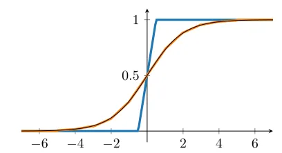
We found the piecewise linear approximation of the sigmoid function introduced in (Mohassel & Zhang,2017)

SIGMOIDAPPROX(x) :=

    

0 ifx_{≤ −}1 2,

x+1₂ if −1 2 < x <

1 2, 1 ifx_≥1

2.

to work best, see Figure4.

Algorithm 1Fair model training with private sensitive val-ues using Lagrangian multipliers forF(θ) =1_/n|Z>_X

| −c. Parties: M, REG.

Input: (M)_hZi1∈Zn×pq Input: (REG)X_∈Zn×d

q ,y∈Znq,hZi2∈Zn×pq

Input: (Public) Learning ratesηθ, ηλ, number of training examplesn, minibatch size2s_{, constraintsc}

∈Zp

q, number of epochsNe.

1: θ_←0,λ_←0

2: A_←BLOCKEDMULTSHIFTAVG(Z>_,X)

3: for alljfrom1toNedo

4: for allifrom1ton_/2s_do

5: (Xi,yi)←SAMPLEMINIBATCH(X,y)

6: F← |Aθ_{| −}c

7: ∇λ←max{F,0}

8: σ←SIGMOIDAPPROX(Xiθ)

9: _∇BCE

θ ←SHIFTDIVIDE(X>i (σ−yi),2s)

10: _∇CON

θ ←

    

A>_{λ, ifA>0}

∧F>0 −A>_{λ, ifA<0}

∧F>0 0, ifF≤0

11: θ_←θ₋ηθ(ξjBCE∇BCEθ +ξjCON∇CONθ )

12: λ_←max_{λ+ηλ∇λ,0}

13: end for

14: end for

Output: Parametersθ

B.2. Description of Training Parameters

All our experiments use a batch size of 64, a fixed number of epochs scaling inversely with dataset sizen(such that

−6 ₋4 ₋2 2 4 6 0.5

1

Figure 4.Piecewise linear approximations for the non-linear

sig-moid function (in black) fromMohassel & Zhang(2017) in blue and fromFaiedh et al.(2001) in orange.

schedule for 1_/tin the interior point logarithmic barrier method as described byBoyd & Vandenberghe(2004). The weights for the gradients of the regular binary cross entropy loss (BCE) and the loss from the constraint terms (CON) follow the schedules

ξjBCE=

Ne

Ne+j , ξ

CON

j =

Ne+ 10j

Ne .

Weight decay, adaptive learning rate schedules. and momen-tum neither consistently improved nor impaired training. Therefore, all reported numbers were achieved with vanilla SGD, for fixed learning rates, and without any regulariza-tion. After extensive testing on all datasets, we converged to a fixed-point representation with 16 bits for the integer and fractional part respectively. The smaller the number of bits, the faster the MPC implementation and the higher the risk of loss of precision or over- and underflows. We found 16 bits to be the minimally needed precision for all our experiments to work.

C. Additional Experimental Results

C.1. Results on Remaining Datasets

Analogously to Figures2and Figure3we report the results on test accuracy as well as the mitigation of disparate impact for the Lagrangian multiplier method in Figure5. In the Adult dataset we are able to mitigate disparate impact with slightly worse accuracy as compared to the baseline. Note that the German dataset contains only 512 training and 200 test examples, which explains the discrete jumps in accuracy in minimal steps of1_{/200= 0.}005. Hence, even though the Lagrangian multiplier technique here consistently removes disparate impact to a similar extent as the baseline, interpre-tations of results on such small datasets require great care. For the much larger stop, question and frisk dataset we again observe the curious initial increase in accuracy similar to our observations for the Bank dataset. In this dataset about 93%of all samples have positive labels, which explains the near optimal accuracy when collapsing to always predict 1,

which happens for the baseline as well for our method at a similar rate ascdecreases.

C.2. Disadvantages of Other Optimization Methods

In Section5we suggest the Lagrangian multiplier technique for fair model training using fixed-point numbers. Here we substantiate this suggestion with further empirical evidence. Figure6shows analogous results to Figure3and the second row of Figure5. These plots reveal the shortcomings of the interior point logarithmic barrier and the projected gradient methods.

Interior Point Logarithmic Barrier method. While the interior point logarithmic barrier method does balance the fractions of people being assigned positive outcomes be-tween the two different demographic groups when the con-straint is tightened, it soon breaks down entirely due to overflow and underflow errors. The number of failed runs was substantially higher than for the Lagrangian multiplier technique. As explained in (Boyd & Vandenberghe,2004), when we increase the parametertof the interior point loga-rithmic barrier method during training, the barrier becomes steeper, approaching the function

I−(x) =

(

0 forx_≤0,

∞ forx >0.

From this it becomes obvious that when facing tight con-straints, the gradients might change from almost zero to extremely large values within a single update of the pa-rameters θ. Moreover, iplb requires careful tuning and

scheduling oft. Hence, the interior point logarithmic barrier method, while achieving good results over some domains, is not well suited for MPC.

Projected gradient method. In Figure6, we observe that the projected gradient method seems to fail in most cases, since it does not actually balance the fractions of positive outcomes across the sensitive groups. There is a simple explanation why it can satisfy the constraintF(θ)_≤0for thep%-rule even with smallcand still retain near optimal accuracy. Note that the accuracy only depends on the direc-tion ofθ, i.e., it is invariant to arbitrary rescaling ofθ. Since

the constraint_F(θ) =_|Aθ_{| −}c_≤0is always satisfied for

θ = 0, dividing anyθby a large enough factor will result

in a classifier that achieves equal accuracy and satisfies the constraint (by continuity). However, minimizing the loss in the original logistic regression optimization problem (or equivalently maximizing the likelihood), which is not in-variant under rescaling ofθ, counteracts shrinkingθas it

enforces high confidence of decisions, i.e., largeθ. The

0.8 0.82 0.84

accurac

y

Adult

0.68 0.7 0.72 0.74 0.76

German

0.93 0.94 0.95 0.96

SQF

10−4 10−2 100

0.1 0.2 0.3 0.4 0.5

constraintc

fraction

with

ˆ

y

=

1

10−4 10−2 100

0.7 0.8 0.9

constraintc 10

−4 ₁₀−2 ₁₀0

0.85 0.9 0.95 1

constraintc

Figure 5.First row:The color code isblue: iplb,orange: projected,green: Lagrangewithcontinuouslines for no approximation and

dashedlines for piecewise linear approximation. The gray dotted line is the baseline and the dashed black line marks unconstrained

logistic regression.Second row:Continuous/dottedlines correspond toz= 0anddashed/dash-dottedlines toz= 1. The color code is

(red: no approx. + float,purple: no approx. + fixed,yellow: pw linear + float,turquoise: pw linear + fixed, gray: baseline).

iplb

Synthetic _{COMPAS Bank Adult German} SQF

10−3 ₁₀−1

constraintc

projected

10−3 ₁₀−1

constraintc

10−3 ₁₀−1

constraintc

10−3 ₁₀−1

constraintc

10−3 ₁₀−1

constraintc

10−3 ₁₀−1

constraintc

Figure 6.We plot the fraction of people withz= 0(continuous/dotted) and withz= 1(dashed/dash-dotted) who get assigned positive

outcomes over the constraintcfor 5 different datasets. The different colors correspond to (red: no approximation + floats,purple: no

by the truep%-rule instead of the computational proxy. It also often fails for small constraint values, as the projec-tion matrix in eq. (10) turns out to become near singular producing over- and underflow errors.

D. Clarification of Privacy or Secrecy