doi:10.4236/ica.2011.21006 Published Online February 2011 (http://www.SciRP.org/journal/ica)
Optimal Risk-Sensitive Filtering for System Stochastic of
Second and Third Degree
Ma Aracelia Alcorta-Garcia, Sonia Gpe Anguiano Rostro, Mauricio Torres Torres
Department of Physical and Mathematical Sciences, Autonomous University of Nuevo Leon, Cd. Universitaria, San Nicolas, Mexico
E-mail: [email protected], [email protected], mautor2@gmail.com Received October 9, 2010; revised February 8, 2011; accepted February 10,2011
Abstract
The risk-sensitive filtering design problem with respect to the exponential mean-square cost criterion is con-sidered for stochastic Gaussian systems with polynomial of second and third degree drift terms and intensity parameters multiplying diffusion terms in the state and observations equations. The closed-form optimal fil-tering equations are obtained using quadratic value functions as solutions to the corresponding Focker- Plank-Kolmogorov equation. The performance of the obtained risk-sensitive filtering equations for stochastic polynomial systems of second and third degree is verified in a numerical example against the optimal po-lynomial filtering equations (and extended Kalman-Bucy for system popo-lynomial of second degree), through comparing the exponential mean-square cost criterion values. The simulation results reveal strong advan-tages in favor of the designed risk-sensitive equations for some values of the intensity parameters.
Keywords:Optimal Nonlinear Filtering, Risk-Sensitive Filtering, Extended Kalman-Bucy Filtering
1. Introduction
Since the linear optimal filter was obtained by Kalman and Bucy (60’s), numerous works are based on it, see for example [1-5], of the variety of all those. The determi-nistic filter model introduced by Mortensen [6] provides an alternative to stochastic filtering theory. In this model, errors in the state dynamics and the observations are modeled as deterministic “disturbance functions”, and an exponential mean-square cost criterion disturbance error is to be minimized. Special conditions are given for the existence, continuity and boundedness of f X t
in the state equation, which is considered nonlinear, and the linear function h X t
in the observation equation. A concept of stochastic risk-sensitive estimator, introduced more recently by McEneaney [7], regard a dynamic sys-tem where f X t
is a nonlinear function, linear ob-servations and existence of parameter multiplying the diffusion term in both equations (state and observa-tions). In [8] were obtained the suboptimal risk-sensitive filtering equations for polynomial systems of third de-gree and applied to the pendulum equations [9], in which the original system was linearized applying Taylor series around the equilibrium point. In [10,11] it is regarded
f X t as nonlinear function. This paper presents an
application of the equations obtained in [10,11] for sin-gular form of f X t
(polynomial of second and third degree).The goal of this work is to obtain the optimal risk- sensitive filtering equations when the form of f X t
is polynomial of second and third degree and parameter multiplying the diffusion term in the state and obser-vations equations. There filtering equations are obtained taking a value function as solution of the nonlinear pa-rabolic partial differential equation and exponential mean-square exponential cost criterion to be minimized.
Undefined parameters in the value function are calcu-lated through ordinary differential equations composed by collecting terms corresponding to each power of the state-dependent polynomial in the nonlinear parabolic PDE equations. This procedure leads to the obtention of the optimal risk-sensitive filtering equations.
polynomial filtering equations (and extended Kalman- Bucy for systems of second degree), through comparing the exponential mean-square cost criterion values in fi-nite horizon time. The simulation results reveal strong advantages in favor of the designed risk-sensitive filter-ing equations for all values of the intensity parameters (in Table 1) multiplying diffusion terms in state and
ob-servation equations. Tables of the criterion values and graphs of the simulations are included. This exponential mean-square cost criterion function contains the parame-ter which appear in the dynamic system, which leads to a more robust solution. This work is organized as fol-lows: filtering problem statement, optimal risk-sensitive filtering for stochastic system of second degree, optimal risk-sensitive filtering for stochastic system of third de-gree, application for systems of second dede-gree, applica-tion for systems of third degree, conclusions and refer-ences.
2. Filtering Problem Statement
Consider the following stochastic model (1), where X t
denotes the state process, Y t
denotes a continuousaccumulated observations process, X t
satisfies thediffusion model given by
2 2
dX t f X t dt dW t
(1)
where f X t
represents the nominal dynamics, and W is a Brownian motion, and the observation process
Y t satisfies the equation:
2 2
,
0 0,dY t h X t dt dW t Y
(2)
where is a parameter and W and W are
independ-ent Brownian motions, which are also independindepend-ent of the initial state X
0 . X
0 has probability density
1
exp 0
k X for some constant k.
Let us consider
0
1
log exp T , ,
J E L X t m t t dt Y t
(3)the exponential mean-square cost criterion to be mini-mize. In the rest of the paper the assumptions (A1)-(A4) (from [10]) are hold:
● (A1) , , n
f g h with fx,hx bounded.
● (A2) D1
x2 1
x D2
x21
. Here fx isthe matrix of partial derivatives of f with hx defined
similarly.
x is a continuous, real-valued functionsatisfying (A2) for some positive D1, D2. ● (A3) , n
f h with f, h bounded and fxx, hxx bounded
and globally Hölder continuous. (A function u is globally
Hölder continuous if there exists
0,1 ,
K suchthat u x
u y K xy for all x y, ).● (A4) Given R , there exists KR such that
x y KR x y for all x, y .
Let q T X t
,
denotes the unnormalized condi-tional density of X T
, given accumulatedobserva-tions Y t
for 0 t T . It satisfies the Zakaistochas-tic PDE, in a sense made precise, for instance in [12]. It is assumed that
1
1
0, exp ,
, , exp ,
q X t X t
q T X t p T X t Y T h x t
(4)
where p T X t
,
is called pathwise unnormalized filter density. p satisfies the following linear second- order parabolic PDE with coefficients depending on
Y t :
*.
p K
L T p p
T
(5)
where, for every n
g , let
2
, 2
1 ,
2
1
2
g XX X
X X
X X
L tr ag f g L T g Lg a Y T h g
K T X t a X t Y T h Y T h L Y T h h
(6)
L denotes the differential generator of the Markov dif-fusion X t
in (1). By assumptions (A1) and (A3) in[10], K is bounded and continuous.
L T
* is the for-mal adjoint of L T
. Since Y
0 0, p
0,X t
0,
q X t . The initial condition for (5) is (4). For some given YC0
0,T
, (where C0 denote the spaceof continuous Y t
such that Y
0 0, with the sup norm ). The pathwise filter density p is the unique “strong” solution to (5) and (4) in a sense made precise in [12]. Further, p is a classical solution to (5) and (4) with p continuous on
0, 1
n
T and partial derivatives
, , , , 1, ,
i i j
T X X X
p p p i j n continuous for 0 T T1
[13,14].
Moreover, p T X t Y
,
;
0. We rewrite (5) as fol-lows:
1
2 XX X
p B
tr a X t p A p p
T
(7)
where
X
X
A f X t a X t Y t h x t div a t
(8)
,
49
2 2 ( ( )) , , XX Xtr a X t
div f X t a X t Y T h X t K T X t
, 1 , 1, 1, ,
i
i j
n
X j i j ij X
n
XX i j ij X X
div a t a j n
tr a a
These assumptions imply uniform bounds for A and B, depending on the sup norm Y on
0,T1
, but not on. Taking log transform: Z T X t
,
logp T X t
,
, which satisfies the nonlinear parabolic PDE:
1 ,2 XX X 2 X X
Z
tr Z A Z Z Z B
T
(9)
with initial condition ZX
0,X t
X t
. The optimal risk-sensitive filtering problem consists in found the estimate C t
, of the state X t
through verifica-tion that
1 , 2 , TZ T X t X t C t Q t X t C t T Y T h X t
(10)
is a viscosity solution of (9). Where
n,X t w t
m, Y t
, v t
p, ,f hn with fX, hx bounded is assumed through-
out. Here hx is the matrix of partial derivatives of h and the same form for ZX.
3. Optimal Risk-Sensitive Filtering Problem
3.1. Optimal Risk-Sensitive Filtering for Stochastic System of Second Degree
Taking f X t
A t
A t X t1
A t2
XT
t X t ,
1
h X t E t E t X t with A t
n, A t1
Mn n,
2 n n n,
A t T
1
,p
E t E t Mn p where Mi j
denotes the field of matrixes of dimension ij and
i j k
T denotes the field of tensors of dimension i j k n. The following stochastic equations system is obtained:
1 2 1 t , , TdX A t A t X t A t X t X t dB t
dY t E t E t X t dB t (11)
where
22 . The optimal filtering problemcon-sists in to obtain the estimate of the state X t
given the observations equations, which minimizes theexpo-nential mean-square cost criterion, taking Z T X t
,
(10) as solution of the nonlinear parabolic partial differ-ential Equation (9).Theorem1. The solution to the filtering problem, for
the system (11) with criterion (3) takes the form:
1 1 1 1 1 2 1 1 1 1 2 , . T T TC t A t A t C t Q t Q t C t Q t E t dy E t Q t C t
A t Q t
Q t A t Q t Q t A t Q t Q t E t E t
(12)
where C t
is the state estimate vector with initialconditions with initial condition C
0 C0, and Q t
is a symmetric matrix negative defined, where the initial condition Q
0 q0 is derived from initial conditionsfor Z. If
X t
XT
t KX t
, 0Q K. Proof: The value function is proposed
1 , ( ) 2 , TZ T X t X t C t Q t X t C t T Y T h X t
(13)
0,
, , ,
X
Z X t X t C t Q t t are func-tions defined on
0, ,
n,
T C t Q t is a symmetric matrix of dimension n n and ( ) t is a scalar func-tion) as a viscosity solution of the nonlinear parabolic PDE (9). ZX,ZXX are the partial derivatives of Z
re-spect to X t
and Z is the gradient of Z. Then the partial derivatives of Z are given by:
1 1 1 2 1 2 1 , 2 . T T T X T XXZ X t C t Q X t C t
X t C t Q t C t t
Y t E t E t X t
Z Q t X t C t
X t C t Q t Y t E t
Z Q t
(14)
Let us consider:
1 2 1 TA A t A t X t A t X t X t
Y T E t
(15)
22 1 1
1 2 2 1 1 1 2 2 – 1 2 T
B A t X t A t Y T E t
A t A t X t A t X t X t
Y T E t E t E t X t
Substituting (14) and the expressions for A, B in (9); we obtain:
1 1 2 1 1 1 1 21 1 2
1 0 2 2 1 1 2 2 1 1 2 2 1 2 1 2 T T T T T T
X t C t Q t X t C t Q t C t
t Y t E t E t X t tr Q t
A t A t X t A t X t X t Y t
E t Q t X t C t X t C t
Q t Y t E t Q t X t C t
X t C t Q t Y t E t A t
Y t E t A t A t X t A t X
21 1
1
.
2
t
X t Y t E t E t E t X t
(16) Collecting the T
, T
T
X t X t X t X t X t and
T T
X t X t X t X t terms, and replacing X t
by C t
; we obtain the matrix equation for Q t
.Col-lecting the X t
terms, the vectorial equations for
C t are obtained (12).
3.2. Optimal Risk-Sensitive Filtering for Stochastic System of Third Degree
Taking
1
2
Tf X t A t A t X t A t X t X t
3 ,
T T
A t X t X t X t
h X t
E t
E t X t1
with
n,A t A t1
Mn n,A t2
Tn n n , A t3
Tn n n n ,
p,E t E t1
Mn p where Mi j denotes the fieldof matrixes of dimension ij, Ti j k denotes the field
of tensors of dimension i j k and Ti j k l denotes the field of tensors of dimension i j k l. The
fol-lowing stochastic equations system is obtained:
1 2 3 1 0 t A ,, ,0
T
T T
dX t A t X t A t X t X t
A t X t X t X t dB t
dY t E t E t X t dB t X X
(17)
where
22 .Theorem 2. The solution to the filtering problem, for
the system (17) with criterion (3) takes the form:
1 1 1 1 1 , 2C t A t A t C t Q t Q t C t
Q t E t dy E t Q t C t
(18)
1 1 2
2 2
T
T
Q t A t Q t Q t A t A t Q t C t A t Q t C t A t Q t C t
3 3 3 3 1 1 1 T T T T T T T TA t C t C t Q t A t C t C t Q t A t Q t C t C t
A t Q t C t C t
Q t Q t div f C Y t E t E t E t
where C t
is the state estimate vector with initial conditions with initial condition C
0 C0, and Q t
is a symmetric matrix negative defined, where the initial condition Q
0 q0 is derived from initial conditions for Z. If
T
, 0X t X t KX t Q K
.
Proof: In similar form to Theorem 1.
4. Applications
4.1. Application for Systems of Second-Degree. Optimal Risk-Sensitive Filtering Equations
Consider the following dynamical stochastic system as-sociated to a continuous stirred tank reactor in which is a chemical reaction occurs. This reaction is in liquid phase and has isothermal character between multicomponents [15].
1 1 1 2 1
2
2 1 1 2 2 2 2 2
1 , 2 . 2 a a a
X t D X u t dW t
X t D X X D X dW t
(19)
where X1
t represents the unnormalizedconcentra-tion P CPo of a certain specie P of the reactor, X2
trepresents unnormalized concentration CQ CPo of a
certain specie Q. The control variable u is defined as the relation between the alimentation molar rate by volumet-ric unit of P, designated by NPF and the nominal
con-centration CPo, this is uNPF FCPo , where F is the
volumetric flow of alimentation on 3 1
m s . Da1k V F1 ,
2 2
a Po
D k VC F where V is the volume of reactor in 3
m , k1 and k2 are constants of first degree given in 1
s . It can take that Da1 and Da2 are considering by
1 1
a
D and Da2 1. Q is highly sour while P is neuter. Then, the following dynamical stochastic system is ob-tained:
1 1 2 1
2
2 1 2 2 2 2
2 ,
2
. 2
X t X u t dW t
X t X X X dW t
51
Applying the equations (12) to the system (20), the equations of the optimal risk-sensitive filtering are ob-tained:
2 2
11 11 11 12
12 12 11 11 12 12 22
2 2
22 22 12 12 22
11
1 2 11 22 1 12 2
11 22 12
12 11 2 12 1 1 22 2 12
1 11 1 12 2
12
2 2 12 2
11 22 12
4 1,
3
2 2 1,
,
2 ,
Q Q Q Q
Q Q Q Q Q Q Q
Q Q Q Q Q
Q
C Q Q C Q C
Q Q Q
Q Q C Q C Y Q Y Q C Q C Q C
Q
C Q Q
Q Q Q
2 1 12 2
22 11 2 12 1 1 12 2 11 11
1 2 12 1 22 2
.
2
C Q C
Q Q C Q C Y Q Y Q Q
C C Q C Q C
(21)
The initial conditions for the risk-sensitive filtering equations are: X1
0 20,X2
0 10,Y1
0 2,Y2
0 1,
1 0 1,
C C2
0 5, Q11
0 6, Q12
0 0.0001,
22 0 7
Q , the final time is T 2s . The system formed by the equations (20) and (21), is simulated using Simulink in MatLab7. The performance of the designed equations is compared versus the equations of the poly-nomial filtering [1] and the equations of the extended Kalman-Bucy filtering [16], applied to the system (20), that is optimal with respect to the conventional exponen-tial mean-square cost criterion.
4.1.1. Polynomial Filtering Equations
The corresponding equations for the polynomial filtering [1] are given by:
2 2 211 11 2 12 11
2
12 11 12 2 12 11 12 12 22
2
2 2
22 22 12 2 22 2 12 22
2
1 1 11 1 1 12 2 2
2
2 1 1 2 22
2
12 1 1 22 2 2
2
4 ,
2
2
3 2 ,
2
2 2 4 ,
2 2
2 ,
2
.
P P P P
P P P m P P P P P
P P P m P P P
m m P Y m P Y m
m m m m P
P Y m P Y m
(22)
where the initial conditions are X1
0 20, X2
0 10,
1 0 2,
Y Y2
0 1, m1
0 1, P11
0 100, P12
0 1,
722 0 1 10
P .
4.1.2. Extended Kalman-Bucy Filtering Equations
The equations of the extended Kalman-Bucy [13] filter-ing are given by:
2 2 211 2 12 11
2
12 11 12 11 12 12 22
2
2 2
22 12 22 2 12 22
2
1 1 11 1 1 12 2 2
2 4 , 2 2 3 , 2
2 2 ,
2 2
2 ,
P P P P
P P P P P P P
P P P P P
m m P Y m P Y m
(23)
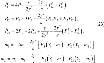
22 1 1 12 1 1 22 2 2
2
.
m m m P Y m P Y m
1) Consider the stochastic dynamical system associ-ated to a continuous stirred tank reactor and the follow-ing initial conditions for the state and observations equa-tions: X1
0 20, X2
0 10, 0Y1
2, Y2
0 1, thefinal time is T 2s. The initial conditions for the
fil-tering equations in which case are given by: a) For risk-sensitive filtering equations:
1 2 11 12
22
0 1, 0 5, 0 6, 0 0.0001,
0 7.
C C Q Q
Q
b) For polynomial filtering equations:
1 2 11 12
7 22
0 1, 0 5, 0 100, 0 1,
0 1 10 .
m m P P
P
c)For Extended Kalman-Bucy filtering equations:
1 2 11 12
22
0 1, 0 5, 0 5, 0 3,
0 5.
m m P P
P
[image:5.595.324.537.123.251.2]
Table 1 presents comparison between the exponential
mean square cost criterion J for the three types of filter-ing equations; you can see that the JR S values are the
smallest for all values of the intensity parameter . 2) Consider the stochastic dynamical system associ-ated to a continuous stirred tank reactor and the follow-ing initial conditions for the state and observations equa-tions: X1
0 50, X2
0 1, 0Y1
2, 0Y2
1, thefinal time is T 2s. The initial conditions for the
fil-tering equations in which case are given by: a) For risk-sensitive filtering equations:
1 2 11 12
22
0 1, 0 5, 0 7, 0 0.0001,
0 7.5.
C C Q Q
Q
b) For polynomial filtering equations:
1 2 11 12
7 22
0 1, 0 5, 0 85, 0 10
.
,
0 2 10
m m P P
P
c) For Extended Kalman-Bucy filtering equations:
1 2 11 12
22
0 1, 0 5, 0 2, 0 5, 0 10.
m m P P
P
Table 2 presents comparison between the exponential
mean square cost criterion J for the three types of filter-ing equations; you can see that the JR S values are the
smallest for all values of the intensity parameter . 3) Consider the stochastic dynamical system associ-ated to a continuous stirred tank reactor and the follow-ing initial conditions for the state and observations equa-tions: X1
0 0.05, X2
0 50, 0Y1
2, Y2
0 1,the final time is T 2s. The initial conditions for the
filtering equations in which case are given by: a) For risk-sensitive filtering equations:
1 2 11 12
22
0 1, 0 5, 0 6, 0 0.0001,
0 7.
C C Q Q
Q
b) For polynomial filtering equations:
1 2 11 12
7 22
0 1, 0 5, 0 100, 0 5,
0 1 10 .
m m P P
P
c) For Extended Kalman-Bucy filtering equations:
1 2 11 12
22
0 1, 0 5, 0 1.85, 0 3,
0 5.
m m P P
P
Table 3 presents comparison between the exponential
mean square cost criterion J for the three types of filter-ing equations; you can see that the JR S values are the
smallest for all values of the intensity parameter . With these tables, showed that the filter risk-sensitive is the best, because the values obtained are lower.
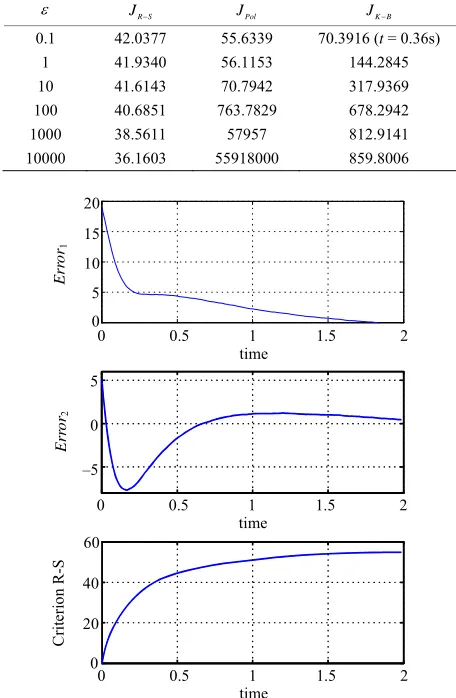
The Figures 1, 2 and 3 show the Error1 and Error2
which are defined as Error1 X1
t C t1
(in sameform for Error2); and the exponential mean-square cost
[image:6.595.55.287.503.589.2]criterion values in T 2s.
Table 1. Comparison of exponential mean-square cost cri-terion values J(3) in T = 2s for risk-sensitive, polynomial and extended Kalman-Bucy filtering equations.
JR S JPol JK B
0.1 53.4293 69.2292 (t = 0.17s) 69.0816(t = 0.14s)
1 53.5165 145.7323 277.3136
10 53.7994 157.2172 235.5110
100 54.7621 858.7622 189.6937
[image:6.595.56.286.638.722.2]1000 58.5054 58230 185.7343
Table 2. Comparison of exponential mean-square cost cri-terion values J(3) in T = 2s for risk-sensitive, polynomial and extended Kalman-Bucy filtering equations.
JR S JPol JK B
1 505.8493 705.1152 (t = 1.64s) 686.3813 (t = 0.28s)
10 513.3591 712.2522 527.0787
100 537.8120 1430.4728 587.0328
1000 622.1946 59067 641.1202
10000 960.423 5597700 673.6555
Table 3. Comparison of exponential mean-square cost cri-terion values J(3) in T = 2s for risk-sensitive, polynomial and extended Kalman-Bucy filtering equations.
JR S JPol JK B
0.1 42.0377 55.6339 70.3916 (t = 0.36s)
1 41.9340 56.1153 144.2845
10 41.6143 70.7942 317.9369 100 40.6851 763.7829 678.2942
1000 38.5611 57957 812.9141
10000 36.1603 55918000 859.8006
Err
o
r1
Err
o
r2
Cr
iteri
on
R-S
0 0.5 1 1.5 2
time 20
15
10
5 0
0 0.5 1 1.5 2
time
0 0.5 1 1.5 2
time 0
5
–5
60
40
20
0
Figure 1. Graphs of the Error , 1 Error , and exponential 2 mean square cost criterion corresponding to the risk-sensi- tive optimal filtering equations for a continuous stirred tank reactor for 10, X1
0 20, X2
0 10, Y1
0 2,
2 0 1
Y .
4.2. Application for Polynomial System of Third Degree
4.2.1. Optimal Risk-Sensitive Filtering Equations
The risk-sensitive control equations for third degree po-lynomial systems will be applied to the problem of ori-entation of a monoaxial satellite [15]. The description is as follows: a satellite rotates around a fixed axis without gravity. The rotation torques is produced by a system of mini-engines through a controlled explosion of gases in the opposite direction. The state equations for this model are given by:
2
1 0.5 1 1 2 2 2 1
X t X t X t dW t
53
2 2 2 2 , 1 2 2 .
X t dW t Y t X t dW t
(24)
where X1
t represents the orientation angle of thesatellite, measured with respect of a secondary axis which does not coincide with the principal one. X2
trepresents the angular velocity with respect to the prin-cipal axis. Applying the system of equations (18) to the system (24), the following optimal risk-sensitive filtering equations are obtained:
2
11 12 1 2 11 2 12 2 22 11
22 1 2
12 22 11 12 12 22
2 2
22 12 22 1 2
22
1 2 1 11 2 12
11 22 12
12
1 12 2 22 2
2
11 22 12
1 11 2 12
2 , 0.5 , , 1 2 ,
Q Q C C Q C Q C Q Q
Q C C
Q Q Q Q Q Q
Q Q Q C C
Q
C C Q C Q Y
Q Q Q
Q
C Q C Q C
Q Q Q
C Q C Q
C
121 11 2 12
2
11 22 12
11
1 12 2 22 1 12
2
11 22 12
2 22
.
Q
C Q C Q Y
Q Q Q
Q
C Q C Q C Q
Q Q Q
C Q (25) Err o r1 Err o r2 Cr iter io n P O L
0 0.5 1 1.5 2
time 20 12 160 15 10 5 0 9 6 3 0
0 0.5 1 1.5 2
time
0 0.5 1 1.5 2
time 120
80
40
[image:7.595.334.513.78.320.2]0
Figure 2. Graphs of the Error1, Error2, and exponential mean square cost criterion corresponding to the polynomial filtering equations for a continuous stirred tank reactor for
10,
X1
0 20, X2
0 10, Y1
0 2, Y2
0 1.Err o r1 Err o r2 Cr iter io n K-B
0 0.5 1 1.5 2
time 20
12
250
0 0.5 1 1.5 2
time 15 10 5 0 9 6 3 0 200 150 100 50 0
0 0.5 1 1.5 2
time
Figure 3. Graphs of the Error1, Error2, and exponential mean square cost criterion corresponding to the extended Kalman-Bucy filtering equations for a continuous stirred tank reactor for 10, X1
0 20, X2
0 10, Y1
0 2,
2 0 1
Y .
The initial conditions are: X1
0 0.115, X2
0 0.073,
1 0 0,
Y C1
0 0.92, and C2
0 0.5,Q11
0 4500,
12 0 100,
Q Q22
0 8500, T 1.8s.4.2.2. Polynomial Filtering Equations
The corresponding equations for the polynomial filter [1] are given by:
11 12 12 11 12 22 11 1 2
2 2
2 11
12 2 2
2 2 2
11 12 12
12 22 22 2
2
1 2 2 11 1 2
2 11
1 1
2 12
2 1 1
3 3 3
2 3 , 2 2 2 0.5 , , 2
0.5 1.5 0.5
2 , 2 .
P P P P P P P m m
P P m
P P P
P P P
m m m P m m
P
Y m
P
m Y m
(26)
1) Consider the stochastic dynamical system associ-ated to a problem of orientation of a monoaxial satellite and the following initial conditions for the state and ob-servations equations: X1
0 0.09, X2
0 0.65,Y1
0 2,
2 0 1
Y , the final time is T 1s. The initial
[image:7.595.342.540.479.630.2]a) For risk-sensitive filtering equations:
1 2 11 12
22
0 0.92, 0 0.5, 0 400, 0 100, 0 850.
C C Q Q
Q
b) For polynomial filtering equations:
1 2 11 12
22
0 0.92, 0 0.5, 0 10, 0 20,
0 5.
m m P P
P
[image:8.595.308.542.218.311.2]
Table 4 presents comparison between the exponential
mean square cost criterion J for the two types of filtering equations; it can be saw, that the JR S values are the
smallest for all values of the intensity parameter . 2) Consider the stochastic dynamical system associ-ated to a problem of orientation of a monoaxial satellite and the following initial conditions for the state and ob-servations equations: X1
0 0.115, X2
0 0.073,
1 0 2, 2 0 1
Y Y , the final time is T 1s. The initial
conditions for the filtering equations in which case are given by:
a) For risk-sensitive filtering equations:
1 2 11
12 22
0 0.92, 0 0.5, 0 4500, 0 100, 0 8500.
C C Q
Q Q
b) For polynomial filtering equations:
1 2 11
12 22
0 0.92, 0 0.5, 0 1500,
0 879.21, 0 1000.
m m P
P P
[image:8.595.131.504.381.687.2]
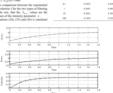
Table 5 presents comparison between the exponential
mean square cost criterion J for the two types of filtering equations; it can be saw, that the JR S values are the
smallest for all values of the intensity parameter . The system Equations (24), (25) and (26) is simulated
using Simulink in MatLab7. The performance of the de-signed equations is compared versus the equations of the polynomial filter [1], with respect to the exponential mean-square exponential criterion J.
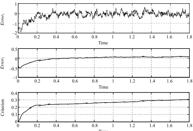
The Figures 4 and 5 show the Error1 and Error2
which are defined as Error1X1
t C t1
(in sameform for Error2); and the exponential mean- square cost
criterion values.
Table 4. Comparison of mean-square exponential criterion J(3) for r-s filtering equations and polynomial filtering eq-uations.
JR S JPol
0.01 0.3239 2.0321
0.1 0.3232 1.1319
1 0.3198 0.6655
10 0.3063 0.3319
100 0.2800 26.8974
Table 5. Comparison of mean-square exponential criterion J(3) for r-s filtering equations and polynomial filtering eq-uations.
JR S JPol
0.01 0.3842 0.5895
0.1 0.3835 0.4287
1 0.3691 0.4013
10 0.2841 0.3054
100 0.1454 0.2454
Err
o
r1
Err
o
r2
Cr
iter
ion
0 0.2 0.4 0.6 0.8 1 1.2 1.4 1.6 1.8
Time 0.5
0.4
0 0.2 0.4 0.6 0.8 1 1.2 1.4 1.6 1.8
Time
0 0.2 0.4 0.6 0.8 1 1.2 1.4 1.6 1.8
Time 0
–0.5
–1
0.5 0.25
0 –0.25
–0.5
0.3 0.2 0.1 0
55
Err
o
r1
Err
o
r2
Cr
iter
ion
0.5
0.4
Time 0
–0.5
0.3
0 0.2 0.4 0.6 0.8 1 1.2 1.4 1.6 1.8
Time
0 0.2 0.4 0.6 0.8 1 1.2 1.4 1.6 1.8
Time
–1 –1
–2 0 1
0.2 0.1 0
[image:9.595.133.462.76.300.2]0 0.2 0.4 0.6 0.8 1 1.2 1.4 1.6 1.8
Figure 5. Graphs of the Error1, Error2, and exponential mean square cost criterion corresponding to the polynomial filter-ing equations for satellite monoaxial for 10, X1
0 0.115, X2
0 0.073, Y1
0 2, Y2
0 1.5. Conclusions
In this paper the equations have been obtained for the optimal risk-sensitive filtering problem, when the system is polynomial of second and third degree, with presence of Gaussian white noise, exponential mean-square cost criterion to be minimized, with parameter multiply-ing the Gaussian white noise in the state and observa-tions equaobserva-tions, and taking into account a value function as a viscosity solution of the nonlinear parabolic PDE.
Numerical application is solved for risk-sensitive and polynomial filtering equations for system of second and third degree (and Kalman-Bucy for system of second degree) for some values of parameter . The perform-ance for optimal risk-sensitive filtering equations is veri-fied through of the comparison between the values of the exponential mean-square cost criterion J for polynomial and extended Kalman Bucy filtering equations.
It can be seen that the values of the mean square cost criterion JR S in final time, are smaller than JPol and
K B
J for all values given to the intensity parameter .
6. References
[1] M. V. Basin and M. A. Alcorta-García, “Optimal Filter-ing and Control for Third Degree Polynomial Systems,”
Dynamics of Continuous Discrete and Impulsive Systems,
Vol. 10, 2003, pp. 663-680.
[2] M. V. Basin and M. A. Alcorta-García, “Optimal Filter-ing for Bilinear Systems and Its Application to Terpo- lymerization Process State,” Proceedings of IFAC 13th
Symposium on System Identification, 27-29 August 2003,
Rotterdam, 2003, pp. 467-472.
[3] F. L. Lewis, “Applied Optimal Control and Estimation,” Prentice Hall PTR, Upper Saddle River, 1992.
[4] V. S. Pugachev and I. N. Sinitsyn, “Stochastic Systems Theory and Applications,” World Scientific, Singapore, 2001.
[5] S. S.-T. Yau, “Finite-Dimensional Filters with Nonlinear Drift. I: A Class of Filters including both Kalman-Bucy and Benes Filters,” Journal of Mathematical Systems, Es-timation, and Control, Vol. 4, 1994, pp. 181-203.
[6] R. E. Mortensen, “Maximum Likelihood Recursive Non- linear Filtering,” Journal of Optimization Theory and Ap-plications, Vol. 2, No. 6, 1968, pp. 386-394. doi:10.1007/
BF00925744
[7] W. M. McEneaney, “Robust H∞Filtering for Nonlinear
Systems,” Systems and Control Letters, Vol. 33, No. 5,
1998, pp. 315-325. doi:10.1016/S0167-6911(97)00124-2 [8] M. A. Alcorta-García, M. V. Basin, S. G. Anguiano and J.
J. Maldonado, “Sub-optimal Risk-Sensitive Filtering for Third Degree Polynomial Stochastic Systems,” IEEE Control Applications & Intelligent Control, St. Petersburg,
8-10 July 2009, pp. 285-289.
[9] H. K. Khalil, “Nonlinear Systems,” 3rd Edition, Prentice Hall, Upper Saddle River, 2002.
[10] W. H. Fleming and W. M. McEneaney, “Robust Limits of Risk Sensitive Nonlinear Filters,” Mathematics of Control, Signals, and Systems, Vol. 14, No. 1, 2001, pp.
109-142. doi:10.1007/PL00009879
[11] W. M. McEneaney, “Max-Plus Eigenvector Representa-tions for Solution of Nonlinear H1Problems: Error Ana- lysis,” SIAM Journal on Control and Optimization, Vol.
[12] D. L. Lukes, “Optimal Regulation of Nonlinear Dynamic Systems,” SIAM Journal on Control and Optimization,
Vol. 7, No. 1, 1969, pp. 75-100. doi:10.1137/0307007 [13] T. Yoshida and K. Loparo, “Quadratic Regulatory Theory
for Analitic Nonlinear Systems with Additive Controls,”
Automatica, Vol. 25, No. 4, 1989, pp. 531-544. doi:10.10
16/0005-1098(89)90096-4
[14] N. N. Ural’ceva, O. A. Ladyzenskaja and V. A.
Solon-nikov, “Newblock Linear and Quasi-Linear Equations for Parabolic Type,” American Mathematical Society, Provi- dence, 1968.
[15] H. Sira-Ramírez, R. Márquez, F. Rivas-Echeverría and O. Llanes-Santiago, “Automática y Robótica: Control de Sistemas no Lineales,” Pearson, Madrid, 2005.