Two dimensional Ising model with Einstein site phonons

L. Pili1 and S. A. Grigera1, 2 1

Instituto de F´ısica de L´ıquidos y Sistemas Biol´ogicos, UNLP-CONICET, La Plata 1900, Argentina 2_{SUPA, School of Physics and Astronomy, University of St Andrews, North Haugh, St Andrews KY16 9SS, UK}

(Dated: April 16, 2019)

We consider a simple Ising magnetic model in two dimensions with Einstein site phonons and study it using Monte Carlo simulations that take into account both degrees of freedom simultaneously. In non-frustrated systems, like the square lattice with ferromagnetic and antiferromagnetic interactions, we find that the coupling of the magnetic to the elastic degrees of freedom gradually lowers the magnetic ordering transition until it is completely suppressed at a critical value of the coupling constant. Above this the system suffers a simultaneous magnetic and structural transition into a

dimerised state with lower crystalline symmetry and ferromagnetic clusters antiferromagnetically aligned. In the case of the Kagom´e lattice with antiferromagnetic interactions, which is frustrated, we show that a similar ordered state takes place when the coupling constant is above a critical value.

I. INTRODUCTION

In every real magnetic material there is an interplay be-tween the magnetic and elastic degrees of freedom. While in many cases this is of no consequence for the magnetic order, and can be neglected, there are a growing num-ber of cases where this interplay is key to understanding the ground state and excitations of magnetic materials. Starting with the theoretical prediction of the so-called ‘spin-Peierls” effect1, a progressive spin-lattice dimeriza-tion occurring at low temperatures, observed experimen-tally for the first time in CuGeO32, there has been a rapidly growing literature that addresses this issue both from theoretical3–10 and experimental11–18 perspectives. Theoretical models have considered classical Ising and Heisenberg models coupled with global Debye distortions (e. g. Ref. 3 or Ref. 10), unconstrained (the bond model of Ref. 6) and Einstein site phonons (e.g. Ref. 8 or Ref. 9) which are a good approximation for systems dominated by optical phonons. Treating both degrees of freedom si-multaneously can be a daunting task. Some simulations exist in the literature3,7,10, but the usual method is to perform a Gaussian integral over the set of displacement coordinates in the partition function. The phonons are then integrated out to obtain an effective spin Hamil-tonian which redresses the exchange constants and can introduce additional interaction terms (see e.g. Ref. 8). Analytical work, or simulations, are then performed on the effective system.

The two-dimensional Ising model is probably the sim-plest magnetic model to show a non-trivial phase transi-tion, and is among the most studied models. Surprisingly there is no work in the literature that describes the case of the 2D-Ising model under Einstein distortions. In this work we do a full Monte Carlo simulation, treating si-multaneously spin and elastic degrees of freedom, of the classical Ising model on the square and kagom´e lattices. Following Ref. 8 we consider Einstein distortions and a linear coupling between both degrees of freedom. The model and the Monte Carlo algorithm used for the simu-lations and the consistency checks performed on our

sys-tem are discussed in Sec. II. A conception usually found in the literature is that distortions are important only in frustrated systems and that their main effect is to help ordering by relief of frustration8,9,19–21. Instead, we find that in the unfrustrated square lattice (Sec. IIIA) this coupling weakens the magnetic ordering transition into the fully polarised state. Upon increase above a criti-cal value the coupling leads to a structural distortion si-multaneous with ordering into a different magnetic state, which we label a checkerboard phase, or CB. This CB phase is a zero-magnetisation state, composed of ferro-magnetic clusters ordered anti-ferroferro-magnetically with re-spect to each other. In the frustrated kagom´e case (Sec. IIIB) we find above a critical coupling an ordered state which shares many similarities with theCBphase.

II. MODEL AND METHODS

For our study we use a simple model that takes into account the coupling between magnetic and elastic de-grees of freedom the so-called Einstein site phonon spin model8. In this model, the sites have independent dis-placements given by a set of independent harmonic os-cillators. Here one is assuming that the most impor-tant lattice distortion contribution is coming from opti-cal phonons. This is a reasonable assumption given that in real materials the active magnetic lattice is usually a sub-lattice of a more complex crystal structure (e.g. the pyrochlore Dy lattice in Dy2Ti2O7). The Hamiltonian is then given by

H/_|J0_|= X <i,j>

J(rij)SiSj+Ke 2

X

i

|ui|2. (1)

the displacements to be sufficiently small compared with the lattice parameter (_|ui_| a) then it is reasonable to expand Jij to a linear dependence on the relative site positionsrij

J(rij) = sgn(J0)(1₋α(rij₋1)), (2)

where α is a dimensionless coupling constant. We will use α as a control parameter to measure the degree of coupling to lattice distortions.

To simulate the elastic distortions we consider polar coordinates,θis treated like a clock model of 360 equally spaced angles and the displacement,ρis chosen randomly in a distribution from 0 to a temperature dependent max-imum δmax(T). The use of the latter has no impact on the results obtained from the simulation, it is introduced merely as a way to optimise the speed of the simulations by avoiding the proposal of extremely unlikely moves at low temperatures. To determine δmax(T) we simu-late a spin-less lattice with a large δmax and calculate a histogram of the displacements at several temperatures. From each of these we choose aδmax(T) such that it in-cludes 80% of the histogram. We then fit a power law to these points and use the fitted function in the simu-lations. The function that fits best has, as expected, a square root dependence inT /J0. A spin-less simulation of a square lattice using this algorithm gives the correct specific heat (Cv = 1) and the correct temperature de-pendence for the mean square displacement (_hu2

i ∝T). In our Monte Carlo simulation we treat simultaneously the magnetic and elastic degrees of freedom using a Born-Oppenheimer (BO) approximation, that is, by assuming that the relaxation times of the magnetic degrees are much shorter than the elastic. Each step of the simu-lation is split into elastic and magnetic moves. The BO approximation translates into the fact that each elastic move is done with a relaxed magnetic configuration. The algorithm proceeds as follows:

We do P elastic Monte Carlo steps (MCS), each of which consists of the following:

1. Choose a random site.

2. Propose a move by picking at random an angle and a displacement (from 0 toδmax).

3. Calculate the exchange constants for the proposed spacial configuration.

4. Calculate the total energy of the system (mag-netic+elastic) and accept or reject the move ac-cording to Metropolis.

5. MakeQmagnetic moves, each move consists of:

(a) Flip one spin at random

(b) Calculate the change in magnetic energy (c) Accept or reject according to Metropolis (d) Repeat (a) to (c) until each spin has been

cho-sen at least once on average.

1 2 3

1.0 1.5 2.0 2.5

Cv

(

α

=

0)

0.0 0.5 1.0 1.5

Cv

(Ising

)

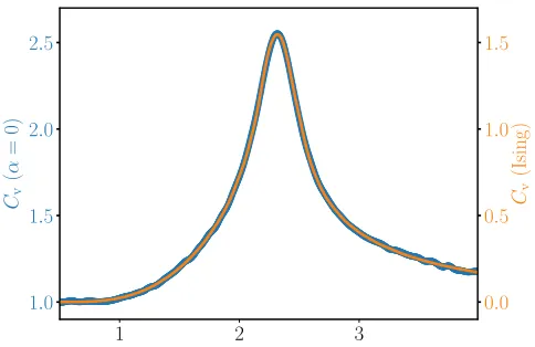
FIG. 1. Comparison between the specific heat of a decoupled elastic system (blue line, left axis) and a static Ising system (orange line, right axis). As expected the specific heat of the former is a simple sum of the elastic contribution (Cel

v = 1)

and the magnetic Ising part (the right axis is shifted accord-ingly in the plot).

6. Repeat 1. to 5. until each site has been chosen at least once on average.

We have checked that our results are independent of the precise choice of the ratioP/Q by running different simulations on lattices withN sites withQvarying from 1 to 300, that is, the number of moves for each Q be-ing fromN to 300N times those for each P. We have used square lattices with L from 4 to 24 and typically with P = 107 MCS. Quantities are averaged over time after a waiting period ofP = 50000 M CS to allow for equilibration(see 22). The figures in this paper are all for L= 16.

The energy scales for magnetic and elastic degrees of freedom can be characterised by the critical temperature of the decoupled Ising system,T0

c, and the melting tem-perature,T∗_{. The latter can be defined in our system by} means of the Lindemann criterion in two dimensions23 (p_hu2_{i ≈0.1), and the former can be determined by} sim-ulating the decoupled magnetic system. Using equipar-tition one gets T∗

≈ |J0_|Ke/200. In order to work in the limit _|u_| 1 one must choose Ke such that Tc0/T∗ 1. For the simulations of this work we have chosenKel= 7200 which meansT∗_/T0

c ≈15.

A simple checkup of the simulation algorithm is to compare the results obtained forα= 0, that is, no cou-pling between elastic and magnetic degrees of freedom with the results obtained from a Metropolis simulation of an Ising model on a fixed lattice. Figure 1 shows such a comparison for the specific heat of a L = 16 square lattice. The orange curve corresponds to the static Ising system. As expected, the decoupled elastic system is sim-ply a sum of the elastic contribution (Cel

1.0 1.5 2.0 2.5

Cv

α/αc

0 1/6 2/6 3/6 4/6 5/6

1 2 3

T /|J0| 0.0

0.5 1.0

h|

M

|i

/

|

Ms

|

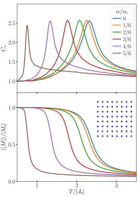
FIG. 2. Specific heat,Cv, (upper panel) and magnetisation,

M, (lower panel) as a function of temperature for a series of fixed values of αbelow αc (see legend). The ferromagnetic

transition progressively moves to lower temperatures asαis increased until it eventually vanishes atαc. The lower panel

shows a snapshot of the ordered state.

III. RESULTS

A. Square lattice

In what follows we will describe the results obtained for ferromagnetic interactions. The antiferromagnetic case can be obtained by the usual mappingSA→ −_SA˜ _{,SB →}

˜

SB, whereAandBare the two disjoint sublattices of the square lattice. We find it useful in terms of presenting the results to separate the discussion for values of α above and below the critical value αc at which the ordering transition vanishes.

1. α < αc: the ferromagnetic transition

Figure 2 shows the specific heat and magnetisation (the order parameter for the FM transition) as a function of temperature as obtained from our simulations for a series

0 1 2

T /_|J0| 0

1 2 3

h

u

i

×10−2

α/αc

0 1/6 2/6 3/6 4/6

5/6 0 1 2

T /|J0|

−1.00

−0.98

h

Jij

i

/

|

J0

|

FIG. 3. Mean value of the displacement,hui, as a function of temperature for differentαbelowαc. In the absence of any

coupling (α= 0) the curve follows the expected√T behaviour (dotted line). For coupled systems the displacement follows the same curve at low temperatures and jumps up at the magnetic transition and follows a √T dependence with an increasingly higher pre-factor (see text). The inset showshJiji

as a function ofT for the same values ofα.

of runs with increasing values of the coupling parameter α. The data shows that the ferromagnetic (FM) transi-tion moves towards lower temperatures asαis increased. As expected, the peak in the specific heat (upper panel) becomes sharper as the critical temperature is reduced, and so does the step towards saturation in the magneti-sation (lower panel). Ifα is further increased, the FM transition temperature sinks towards zero at αc = 60 (for this given value ofKe). A calculation of αc, which becomes clear once the ordered state for high values ofα is known, is given in the appendix.

mag-Jij/_|J 0| −4₋₃

−2_{−1 0}

1 ₂ T/|

J0|

0.0

0.4

0.8

1.2

Coun ts ×10

7

0 1

2

α/αc= 5/6

Jij/_|J

0| −7 ₋₅

−3 ₋

1 1 ₃

5 T/

|J0|

0.0

0.4

0.8

1.2

Coun ts ×10

6

0 2 4 6 8

α/αc= 7/6

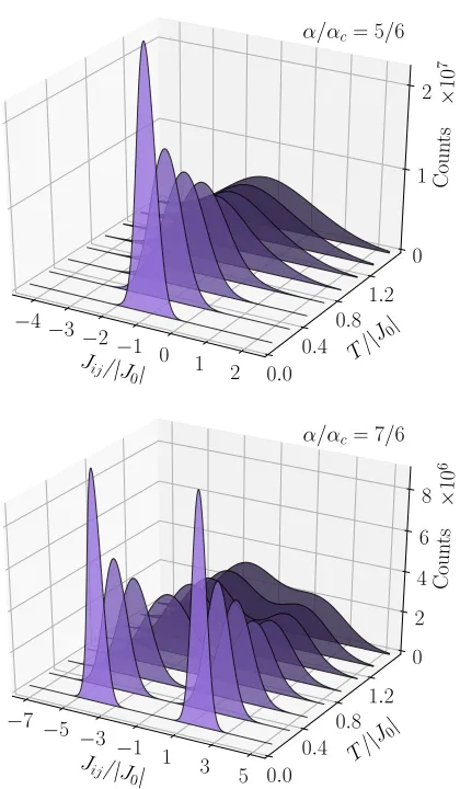
FIG. 4. Histograms for the pair exchange constants, Jij at

different temperatures. In the upper panel for α < αc, and

in the lower panel for α > αc. Below αc the distribution

resembles a Gaussian centred around -1, but closer inspec-tion shows it is skewed to the right at temperatures close to Tc/|J0|= 0.75 (see text for details). Aboveαcit is a bimodal

distribution with two clearly defined F M and AF M peaks that merge as the temperature is raised.

netisation domains. As usual in any Ising transition, the systems start splitting into domains of opposite magneti-sation, but the unusual mechanism in this case is that the antiferromagnetic walls between domains are accompa-nied by distortions that change the sign of the exchange constant and thus render them stable. This mechanism favours the existence of domains of opposite magnetisa-tion of different sizes and thus conspires against theF M order. To ascertain the existence of these two mecha-nisms beyond the mere inspection of snapshots we con-structed a histogram ofJij as a function of temperature. The upper panel of figure 4 shows such a histogram for α/αc = 5/6 using a data window in Jij/|J0| between -20 and -20, with a binning of 0.002, and collecting data over P = 107 MCS. The distribution resembles a Gaus-sian centred aroundJij/_|J0_|=₋1 that increases its

half-0.5 1.0 1.5 2.0

T /|J0|

−1.1 −1.0

h

Jij

i

/

|

J0

|

Mean Max

FIG. 5. The value of Jij at the maximum (green

trian-gles) compared with the mean value,hJiji (blue circles) for

α/αc= 5/6. These should coincide for a symmetric

distribu-tion, instead, there are seen to diverge aboveTc. This is the

evidence of the stabilisation of positive values ofJij around

the domain borders (see text).

maximum width as the temperature is increased. How-ever, a closer inspection reveals that the distribution is slightly skewed towards positiveJij. A quantitative way of seeing this is by comparing the value ofJij at the max-imum with_hJiji, which should coincide for a symmetric distribution. This is shown in figure 5 for α/αc = 5/6. Below the FM transition, Tc(5/6)/_|J0_|= 0.75, both the maximum and the mean value coincide, but atTc there is a jump after which the maximum lies at a consider-ably lower value than the mean. This is evidence of the stabilisation of positive values ofJij around the domain borders. This type of mechanism is particular to the Ising case and should be absent in a Heisenberg system. Indeed, numerical studies of a coupled spin-lattice sys-tem with Heisenberg-like spins show that in this case the transition is only marginally affected by the coupling to vibrations24.

2. α > αc: the checkerboard transition

1 2 3 4

Cv

α/αc

7/6 8/6 9/6

0.5 1.0 1.5 2.0 2.5

T /|J0| 0.0

0.5 1.0

h

Φ

i

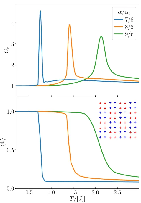
FIG. 6. Specific heat, Cv, (upper panel) and CB order

pa-rameter, Φ, (lower panel) as a function of temperature for a series of fixed values ofα aboveαc (see legend). Increasing

the value of α above αc helps stabilising the CB phase at

progressively higher temperatures. The lower panel shows a snapshot of the ordered state.

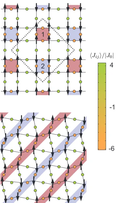
blue to emphasise the checkerboardnature of this state. The pair exchange interactions_hJij_iare shown as circles in the midpoint between bonds, coloured according to the scale shown in the right. The distortions are exaggerated tenfold in the picture for visual clarity.

This state (which we will callCBfor short) is a sort of

dimerisationin two-dimensions: the spins in the clusters are closer to each other (thus enhancing ferromagnetic interactions) and further apart from their neighbours in the other cluster (thus turning this interaction antifer-romagnetic). It is straightforward to notice that theJij show a bimodalF M₋AF Mdistribution, which is readily seen in the histograms for α > αc. An example of these is shown in the lower panel of figure 4, forα/αc = 7/6. Below the transition temperature (Tc(7/6) _≈0.7) there are two separate peaks that evolve into two sharply de-fined identical peaks at low temperatures at ₋4_|J0_| and 2_|J0_|(averaging_−|J0_|).

To characterise this transition it is useful to calculate an order parameter. We use a unit-cell like the one shown

in figure 7. We define an indexjthat runs over all squares in the lattice such that it counts as odd and even the squares marked with 1 and 2 respectively in the picture, and an indexa that runs over the spins in the squares. There are four possible degeneracies of the ground state (plus time reversal), corresponding to where the coloured squares are set in the unit cell. We then define an order parameter Φ that is the sum over the four possibilities, Φ = 1/NP4_m=0(₋1)m

|Φm|, where

Φm= N/4 X

j=1 4 X

a=1

(₋1)jeiφma_σj_{a. (3)}

Here σj

a are Ising-spin variables that can take the val-ues _±1, N is the total number of spins, and the φm a are the phase factors for the spin that take into account the four possible degeneracies: φ1 _{= π(0,0,0,0), φ}2 ₌ π(1,0,1,0), φ3_{=π(1,1,0,0), φ}4_{=π(1,0,0,1).}

The lower panel of figure 6 shows the evolution of the order parameter φas a function of temperature for dif-ferent fixed values ofα(indicated in the figure). As ex-pected, there is a jump inφthat coincides with the peak in the specific heat. The jump is sharp forαclose toαc and softens asα increases. An inspection of the mean value of the displacement _hui, figure 8, shows that the magnetic ordering corresponds with a jump in_hui, i.e., there is a simultaneous magnetic and structural transi-tion. This jump in _hu_i in turn relates with the separa-tion of the peaks in the histogram ofJij that we have discussed earlier. Figure 8 also shows that_hu_iremains non-zero asT →0 aboveαc. It is straightforward to cal-culate_hu(T = 0)_ias the minimum from the two possible ground states (F MandCB). The expression, calculated in the appendix, is simply

umin(α) = (

0 ifα_≤αc √

8

Kelα ifα > αc

. (4)

This is shown as a red line in figure 9 together with the values obtained from the simulations (open circles). As it can be seen there, there is a sharp step in_hu(T = 0)_i atαccorresponding to a structural transition that lowers the lattice symmetry.

4

-1

-6

1

2

FIG. 7. Two snapshots of configurations for α > αc. The

upper panel shows an example of one of the possible checker-boardstates. Here the lattice dimerises into square clusters of equal spin orientation aligned anti-ferromagnetically with re-spect to each other. The dotted line shows the unit cell. The coloured circles correspond to the values of thehJiji in the

bond, and are coloured according to the scale on the right. The lower panel shows astrippedphase. This is a low temper-ature excitation of the CB phase that takes place for values of αclose toαc. For visual clarity, in both cases the distortions

have been exaggerated tenfold.

small distortion configuration, but, as we mentioned be-fore, the distortion in the figure has been multiplied by an order of magnitude to make it apparent.

Similar phases are known to be brought about by cou-pling to lattice distortions in a different context. This is the case of the phonon-induced phases found in the Holstein-Hubbard model25–29. This is model of a cor-related electron system where electron-phonon interac-tions with Einstein phonons are considered in addition to electron-electron interactions. Contrary to our case, this model treats phonons quantum mechanically and has a coupling to elastic degrees of freedom that is odd in nature, since it was originally conceived for a molecular crystal. For large values of the coupling strength, a

bipo-0 1 2

T /|J0| 2.5

3.0 3.5 4.0

h

u

i

×10−2

α/αc

7/6 8/6

0 1 2

T /_|J0|

−1.00

−0.95

h

Jij

i

/

|

J0

|

FIG. 8. Mean value of the displacement, hui, as a function of temperature for differentαaboveαc. The transition into

theCB phase is marked by a jump in huiwhich then inter-ceptsT = 0 at a non-zero value. This is the consequence of a structural transition simultaneous with the magnetic one. The inset shows the mean value of the exchange constant.

0.0 0.5 1.0 1.5 2.0

α/αc

0 1 2 3 4

h

u

(

T

=

0)

i

×10−2

FIG. 9. Distortion atT = 0 as a function of the coupling pa-rameter,α. The blue circles correspond to the values obtained from the simulation, and the red line to those predicted by eq. 4. The sharp step atαc= 60 marks the structural transition.

laronic insulator emerges that is reminiscent of the CB phase found here.

3. T –αphase diagram

FM

PM

CB

FIG. 10. TheT–αphase diagram for the FM Ising model on a square lattice obtained from the simulations. The transitions separate a high temperature paramagnet (PM) from the two ground states: the ferromagnet (FM) and the checkerboard (CB). The single line marks a second-order phase transition while the double line marks first-order. The circles, taken from the position of the peak in the specific heat, show some of the data points used to construct the phase diagram.

simulations. The circles in the figure correspond to the position of the peak in the specific heat.

In the absence of any coupling (α = 0) we find the Ising transition from the high temperature paramagnet (PM) into the ferromagnetically ordered state (FM). This second order transition decreases in temperature asαis increased until it sinks to T = 0 atαc. When the cou-pling is increased beyond this point a new ground state emerges, thecheckerboard (CB), which is a combination of anti-ferromagnetically ordered ferromagnetic clusters. TheCBtransition is simultaneous with a structural tran-sition that decreases the symmetry of the lattice.

As we mentioned, the transition below αc is the ex-pected second order transition in the Ising universality class. This is not the case above αc. The simultane-ous occurrence of the magnetic and structural transi-tions alters the nature of the transition which seems to be first order in the range 1.0 _≤ α/αc .1.3, as deter-mined from the behaviour of the Binder cumulant (not shown)30,31. Some properties show hysteresis in this re-gion when sweeping the temperature up and down. The exact mechanism that determines the range of existence of this first order region is matter of future investigation.

B. Kagom´e lattice

We have applied this same simulation algorithm and data analysis to the case of the Ising model on the Kagom´e lattice. For the F M case the results follow closely those of the square lattice. In the AF M case,

PM

CB

FIG. 11. TheT–αphase diagram for the AFM Ising model on the Kagom´e lattice obtained from the simulations. For low values ofαthere is no long range order at any temperature. Aboveαcthe coupling to the lattice degrees of freedom results

in a lifting of the frustration into a checkerboard (CB) phase at low temperatures. The circles, taken from the position of the peak in the specific heat, show some of the data points used to construct the phase diagram.

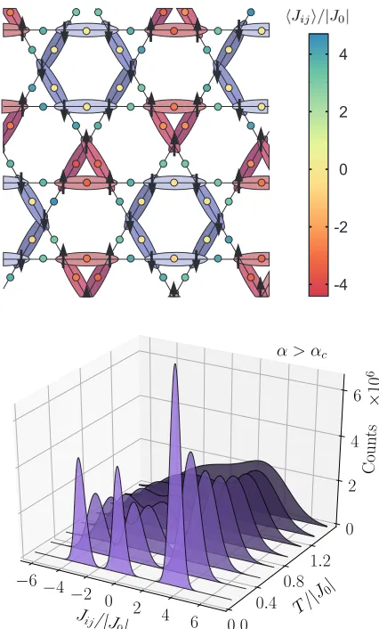
which is frustrated, the systems remains disordered up to a critical value ofαabove which the frustration is lifted through a simultaneous structural and magnetic tran-sition into the kagom´e CB phase (see figure 11). The kagom´e CB , pictured in figure 12, can also be under-stood as a dimerisation along the three different axes of the lattice (pictured as ovals of different shades). How-ever, the distribution of theJij is slightly different, since it is now tri-modal, with two differentF M exchange con-stants corresponding to triangular and hexagonal F M clusters, pictured in the figure in red and blue respec-tively, which are oriented antiferromagnetically with re-spect to each other. This is also a zero magnetisation state, since the number of triangles is twice the number of hexagons.

IV. CONCLUSIONS

4

2

0

-2

-4

J_ij/|J

0| −6₋₄

−_{2 0}

2 ₄

6 T/

|J0|

0.0

0.4

0.8

1.2

Coun ts ×10

6

0 2 4

6

α > αc

FIG. 12. Upper panel: Snapshot of the kagom´e CB. The ovals of different shades mark the dimerisation along the three different directions. The distribution ofJijis in this case

tri-modal, with one AF M peak and two F M constants corre-sponding to the red triangular and the blue hexagonal clus-ters. hJijiis marked by coloured circles located midpoint

be-tween the spins, coloured according to the scale on the right. Lower panel: histogram of the kagom´e CB state obtained from a system ofN = 216 spins showing a trimodal distribution with two peaks at FM couplings and one AFM.

clusters in the kagom´e case. This clusters correspond

to the appearance of a bimodal distribution of exchange constants in the square lattice, one intra-cluster FM and one inter-cluster AFM, and a trimodal distribution in the kagom´e case: two FM interactions (intra-triangles and intra-hexagons) and an AFM interaction inter-cluster. In the unfrustrated case we show that the coupling to the elastic degrees of freedom gradually weakens the transi-tion, through a mechanism whereby domain formation is gradually stabilised by distortions. In the square lattice we identified low-energy excitations consisting ofstripes

of zigzagging spins. The analysis of the phase diagram shows that the transition into the ordered state is not always second order, but further work is needed to iden-tify the exact boundaries and the mechanisms that are responsible for this.

The main aim of this work was to study one of the sim-plest possible models with magneto-elastic coupling, and hence the choice of the Ising model on two-dimensions with linear coupling betweenJandu. It can still be ques-tioned whether such a simple model would have any remit of applicability. Detailed descriptions of the dependence ofJwithuin real materials are scarce. References 32 and 33 provide a careful discussion of the dependence of the magnetic coupling constants of the compound CuGeO3 with respect to lattice distortions. The main magnetic interaction in this case is given by super-exchange paths, but if one makes a simple geometrical model to translate variations in the angle of the mediated pathway into rel-ative displacement between the two magnetic sites, one finds that for the parameters of CuGeO3 displacements in uij of the order of 3% are well described by a lin-ear dependence of J(u) with a coupling constant that varies from 10 to 90 depending on the value chosen for the undistorted angle, i. e. forα/αcbetween 0.16 and 1.5 in the simple Ising model presented here.

ACKNOWLEGMENTS

We are grateful to R. A. Borzi for discussions an a careful read of the manuscript. This work was supported by CONICET (Argentina), and ANPCYT (Argentina) via grant PICT-2013-2004.

1 _{P. Pincus, Solid State Communications9(1971).}

2 _{M. Hase, I. Terasaki, and K. Uchinokura, Physical Review}

Letters70, 3651 (1993).

3 _{L. Gu, B. Chakraborty, P. Garrido, M. Phani, and}

J. Lebowitz, Physical Review B53, 11985 (1996).

4 _{O. Tchernyshyov, R. Moessner, and S. Sondhi, Physical}

review letters88, 067203 (2002).

5 _{O. Tchernyshyov, R. Moessner, and S. Sondhi, Physical}

Review B66, 064403 (2002).

6 _{K. Penc, N. Shannon, and H. Shiba, Phys. Rev. Lett.93,}

197203 (2004).

7 _{C. Weber, F. Becca, and F. Mila, Physical Review B72,}

024449 (2005).

8 _{D. L. Bergman, R. Shindou, G. A. Fiete, and L. Balents,}

Phys. Rev. B74, 134409 (2006) .

9 _{F. Wang and A. Vishwanath, Phys. Rev. Lett.100, 077201}

(2008).

10 _{Y. Shokef, A. Souslov, and T. C. Lubensky, Proceedings}

of the National Academy of Sciences108, 11804 (2011).

11 _{K. Uchinokura, Journal of Physics: Condensed Matter14,}

12 _{H. Ueda, H. A. Katori, H. Mitamura, T. Goto, and H.}

Tak-agi, Physical review letters94, 047202 (2005).

13 _{S. Kimura, M. Hagiwara, H. Ueda, Y. Narumi, K. Kindo,}

H. Yashiro, T. Kashiwagi, and H. Takagi, Physical Review Letters97, 257202 (2006).

14 _{M. Matsuda, H. Ueda, A. Kikkawa, Y. Tanaka, K.}

Kat-sumata, Y. Narumi, T. Inami, Y. Ueda, and S.-H. Lee, Nature physics3, 397 (2007).

15 _{Y. Tanaka, Y. Narumi, N. Terada, K. Katsumata, H. Ueda,}

U. Staub, K. Kindo, T. Fukui, T. Yamamoto, R. Kammuri,

et al., Journal of the Physical Society of Japan76, 043708 (2007).

16 _{R. V. Aguilar, A. Sushkov, Y. Choi, S.-W. Cheong, and}

H. Drew, Physical Review B77, 092412 (2008).

17 _{S. Zherlitsyn, O. Chiatti, A. Sytcheva, J. Wosnitza,}

S. Bhattacharjee, R. Moessner, M. Zhitomirsky, P. Lem-mens, V. Tsurkan, and A. Loidl, Journal of Low Temper-ature Physics159, 134 (2010).

18 _{V. Tsurkan, S. Zherlitsyn, S. Yasin, V. Felea, Y. Skourski,}

J. Deisenhofer, H.-A. K. von Nidda, J. Wosnitza, and A. Loidl, Physical review letters110, 115502 (2013).

19 _{Y. Yamashita and K. Ueda, Phys. Rev. Lett. 85, 4960}

(2000).

20 _{F. Becca and F. Mila, Physical Review Letters89, 037204}

(2002).

21 _{C. Jia and J. H. Han, Physica B: Condensed Matter378,}

884 (2006).

22 _{See Supplemental Material at [URL will be inserted by}

publisher] for a convergence test of the quantities measured in the simulations.

23 _{X. Zheng and J. Earnshaw, EPL (Europhysics Letters)41,}

635 (1998).

24 _{D. Perera, T. Vogel, and D. P. Landau, Phys. Rev. E94,}

043308 (2016).

25 _{M. Capone, G. Sangiovanni, C. Castellani, C. Di Castro,}

and M. Grilli, Phys. Rev. Lett.92, 106401 (2004).

26

P. Werner and A. J. Millis, Phys. Rev. Lett. 99, 146404 (2007).

27 _{J. Bauer and A. C. Hewson, Phys. Rev. B 81, 235113}

(2010).

28 _{Y. Murakami, P. Werner, N. Tsuji, and H. Aoki, Phys.}

Rev. B88, 125126 (2013).

29 _{P. Werner and M. Eckstein, EPL (Europhysics Letters)}

109, 37002 (2015).

30 _{K. Binder, Phys. Rev. Lett.47, 693 (1981).}

31 _{K. Binder, Zeitschrift f¨ur Physik B Condensed Matter43,}

119 (1981).

32 _{M. Braden, G. Wilkendorf, J. Lorenzana, M. Ain,}

G. McIntyre, M. Behruzi, G. Heger, G. Dhalenne, and A. Revcolevschi, Physical Review B54, 1105 (1996).

33 _{R. Werner, C. Gros, and M. Braden, Physical Review B}

59, 14356 (1999).

Appendix: Calculation of the ground state atT = 0

for the square lattice

AtT = 0 it is straightforward to calculate the critical value of the coupling parameter,αc, above which theCB phase is energetically favourable over theF M phase.

We start by calculating the energy in the CB configu-ration. Fig. 13 shows a schematic view of the cell used for this calculation.

b b

b b

b b

b

b

J1 J2

~ui

b b

b b

~rij1 ~rij b

2

FIG. 13. Schematic view of the CB cell used for the calcula-tion of the energy.

Taking the assumption that atT = 0ui~ has identical projections alongxandy and one gets

r1,2ij = 1∓2 u √

2, (A.1)

where u _≡ ui = _|ui~_|. The value of the two exchange constants is then given by

J1,2=J0[1₋α(1_∓2_√u

2 −1)] =J0(1±α √

2u), (A.2)

where we have used thatSiSj =_±1 for 1 and 2 respec-tively.

Thus, the energy per spin of the given unit cell (fig. 13), is given by

εCB= E CB

N =

4J1₋4J2+ 4_|J0_|Kel

2 u 2

4 (A.3)

= 2√2J0α u+_|J0|Kel₂ u2. (A.4)

Minimising the energy with respect to the displacementu one obtains the displacement at minimal energy,umin= √

8_Kα

el, which in turn gives the energy

εCBmin≡εCB(umin) =−4 α2

Kel|J0|. (A.5)

On the other hand, the energy of the FM phase is trivially

εFM min=

EFM min

N =−2|J0|. (A.6)

By equating eqs. A.5 and A.6 one obtains

αc= r

Kel 2 ,

which givesαc = 60 for the parameters used in this work. This is in good agreement with the value determined by the MC simulations.