ISSN Online: 2160-0384 ISSN Print: 2160-0368
DOI: 10.4236/apm.2019.910040 Sep. 30, 2019 832 Advances in Pure Mathematics
The Successive Approximation Method for
Solving Nonlinear Fredholm Integral Equation
of the Second Kind Using Maple
Dalal Adnan Maturi
Department of Mathematics, Faculty of Science, King Abdulaziz University, Jeddah, KSA
Abstract
In this paper, we will use the successive approximation method for solving Fredholm integral equation of the second kind using Maple18. By means of this method, an algorithm is successfully established for solving the non-linear Fredholm integral equation of the second kind. Finally, several examples are presented to illustrate the application of the algorithm and results appear that this method is very effective and convenient to solve these equations.
Keywords
Nonlinear Fredholm Integral Equation of the Second Kind, Successive Approximation Method, Maple18
1. Introduction
The current research intends to the successive approximation method for solv-ing nonlinear Fredholm integral equation of the second kind ussolv-ing Maple18. Homotopy perturbation technique in [1]. A coupling method of a homotopy technique and a perturbation technique [2]. Homotopy perturbation method: anew non-linear analytical technique [3]. Asymptotology by homotopy pertur-bation method [4]. Application of homotopy perturbation method to nonlinear wave equations [5]. Homotopy perturbation method for solving boundary value problems [6]. New interpretation of homotopy perturbation method [7]. Nu-merical Solution of Systems of Linear Volterra Integral Equations Using Block-Pulse Functions [8]. Numerical Analysis and Volterra Integral and Diffe-rential Equations [9] [10]. Biorthogonal Systems for Solving Volterra Integral equation Systems of the Second Kind [11]. Modified HPM for Solving Systems of Volterra Integral Equation of the Second Kind [12]. Analytical and Numerical
How to cite this paper: Maturi, D.A. (2019) The Successive Approximation Method for Solving Nonlinear Fredholm Integral Equation of the Second Kind Using Maple. Advances in Pure Mathematics, 9, 832-843.
https://doi.org/10.4236/apm.2019.910040
Received: August 24, 2019 Accepted: September 27, 2019 Published: September 30, 2019
Copyright © 2019 by author(s) and Scientific Research Publishing Inc. This work is licensed under the Creative Commons Attribution International License (CC BY 4.0).
DOI: 10.4236/apm.2019.910040 833 Advances in Pure Mathematics Methods for Volterra Equations [13]. Numerical Computational Solution of the Linear Volterra Integral Equations System Via Rationalized Hear Functions [14]. Linear and Nonlinear Integral Equation: Methods and Application [15]. Optimal Control Approach for Solving Linear Volterra Integral Equations [16]. Numeri-cal Solution of System of Two Nonlinear Volterra Integral Equations [17] [18]. Adomian Decomposition Method of Fredholm Integral Equation of the Second Kind Using Maple and applications in [19] [20].
Approximate solutions of linear Volterra integral equation systems with variable coeffi cients [21]. Numerical Solution of System of Three Nonlinear Volterra Integral Equation Using Implicit Trapezoidal [22]. Solving nth-Order Inte-gro-Differential Equations Using the Combined Laplace Transfer-Successive Approximations Method [23]. Numerical approach based on Bernstein polyno-mials for solving mixed Volterra-Fredholm integral equations [24]. An inverse eigenproblem and an associated approximation problem for generalized reflex-ive and anti-reflexreflex-ive matrices [25]. Discrete Adomian Decomposition solution of Nonlinear Fredholm Integral Equation [26]. He’s homotopy perturbation method: A strongly promising method for solving non-linear systems of the mixed Volterra-Fredholm integral equations [27]. On the convergence of Ho-motopy perturbation Method [28]. The homotopy perturbation method for solving neutral functional-differential equations with proportional delays [29]. Variational iteration method as a kernel constructive technique [30]. A modified homotopy perturbation method for solving the nonlinear mixed Volter-ra–Fredholm integral equation [31]. A note on the homotopy analysis method [32]. Application of homotopy analysis method to the solution of ninth order boundary value problems in AFTI-F16 fighters [33]. Modeling spectra of break-ing waves propagatbreak-ing over beach [34]. Modified Adomian decomposition me-thod for solving the problem of boundary layer convective heat transfer [35]. New version of Optimal Homotopy Asymptotic Method for the solution of non-linear boundary value problems in finite and infinite intervals [36].
Different types of analytical methods and numerical methods were used to solve the problem [1]-[36]. In this article we have applied the successive ap-proximation method used by using the Maple algorithm by applying this algo-rithm to different examples, including finding the approximate solution and then comparing it to the exact solution and finding out the amount of error be-tween the approximate solution and the exact solution.
The main objective of this work is to use the successive approximations method in solving the nonlinear Fredholm integral equation of the second kind using Maple18.
The paper is arranged as follows: In Section 2, the successive approximations method. In Section 3, numerical examples are also considered to show the ability of the proposed method, and the conclusion is drawn in Section 4.
2. The Successive Approximation Method
DOI: 10.4236/apm.2019.910040 834 Advances in Pure Mathematics
( )
( )
ab( )
,(
( )
)
du x = f x +
λ
∫
K x t F u t t (1)where u x
( )
is the unknown function to be determined, K x t( )
, is the kernel,( )
(
)
F u t is a nonlinear function of u t
( )
, and λ is a parameter. u x0( )
= anyselective real valued function,
( )
( )
( ) ( )
1 , d , 0.
b
n a n
u+ x = f x +
λ
∫
K x t u t t n≥ (2)The question of convergence of u xn
( )
is justified by noting the following theoremTheorem 1 see [16] If f x
( )
in (1) is continuous for the interval a x b≤ ≤and the kernel K x t
( )
, is also continuous in the triangle a x b≤ ≤ , a t b≤ ≤the sequence of successive approximations u x nn
( ),
≥0 converges to the solu-tion u x( )
of the integral equation under discussion.3. Numerical Examples
In this section, we solve some examples, and we can compare the numerical re-sults with the exact solution.
Example 1. Consider the nonlinear Fredholm integral equation of the second kind
( )
( )
2 2( )
0
1
cos d ,
48 12
u x = x −π +
∫
πtu t t(3)
with the exact solution u x
( )
=cos( )
x .Example 2. Consider the nonlinear Fredholm integral equation of the second kind
( )
1 2( )
0
143 1
ln d ,
144 36
u x = x+ +
∫
tu t t(4) [image:3.595.208.539.522.723.2]
with the exact solution u x
( )
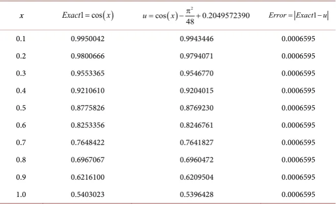
= +x lnx.Table 1. Numerical results and exact solution of Nonlinear Fredholm integral equation of the second kind for example 1.
x Exact1 cos=
( )
x cos( ) 2 0.2049572 98 3
4 0
u= x −π + Error Exact u= 1−
0.1 0.9950042 0.9943446 0.0006595
0.2 0.9800666 0.9794071 0.0006595
0.3 0.9553365 0.9546770 0.0006595
0.4 0.9210610 0.9204015 0.0006595
0.5 0.8775826 0.8769230 0.0006595
0.6 0.8253356 0.8246761 0.0006595
0.7 0.7648422 0.7641827 0.0006595
0.8 0.6967067 0.6960472 0.0006595
0.9 0.6216100 0.6209504 0.0006595
DOI: 10.4236/apm.2019.910040 835 Advances in Pure Mathematics
[image:4.595.205.540.330.708.2]Figure 1. The exact and approximate solutions result of Nonlinear Fredholm integral equation of the second kind.
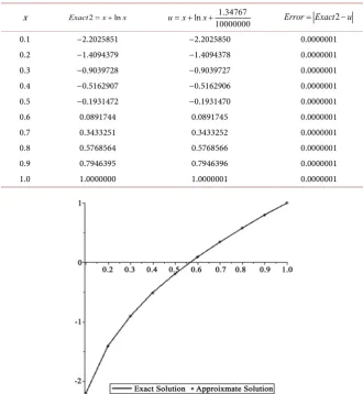
Table 2. Numerical results and exact solution of Nonlinear Fredholm integral equation of the second kind for example 2.
2
Error Exact= −u
1.34767 ln
10000000
u x= + x+
2 ln
Exact = +x x x
0.0000001 −2.2025850
−2.2025851 0.1
0.0000001 −1.4094378
−1.4094379 0.2
0.0000001 −0.9039727
−0.9039728 0.3
0.0000001 −0.5162906
−0.5162907 0.4
0.0000001 −0.1931470
−0.1931472 0.5
0.0000001 0.0891745
0.0891744 0.6
0.0000001 0.3433252
0.3433251 0.7
0.0000001 0.5768566
0.5768564 0.8
0.0000001 0.7946396
0.7946395 0.9
0.0000001 1.0000001
1.0000000 1.0
[image:4.595.206.537.331.690.2]DOI: 10.4236/apm.2019.910040 836 Advances in Pure Mathematics Example 3. Consider the nonlinear Fredholm integral equation of the second kind
( )
(
2)
1 2( )
0
1 1
e 3 e d ,
288 36
x
u x =x − + x+
∫
xtu t t (5)with the exact solution
u x
( )
=
x
e
x.Example 4. Consider the nonlinear Fredholm integral equation of the second kind
( )
(
2)
1(
2( )
)
0
1 1
e 127 e d ,
144 36
x
u x = + − +
∫
t u u t+ t (6) [image:5.595.208.540.272.693.2]with the exact solution
u x
( )
= +
1 e
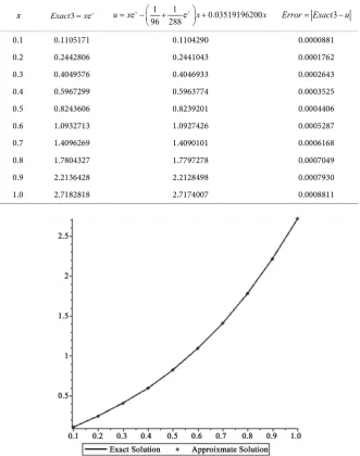
x.Table 3. Numerical results and exact solution of Nonlinear Fredholm integral equation of the second kind for example 3.
3
Error Exact u= −
1 1
e e 0.03519196200
96 288
x x
u x= − + x+ x
3 ex
Exact =x
x
0.0000881 0.1104290
0.1105171 0.1
0.0001762 0.2441043
0.2442806 0.2
0.0002643 0.4046933
0.4049576 0.3
0.0003525 0.5963774
0.5967299 0.4
0.0004406 0.8239201
0.8243606 0.5
0.0005287 1.0927426
1.0932713 0.6
0.0006168 1.4090101
1.4096269 0.7
0.0007049 1.7797278
1.7804327 0.8
0.0007930 2.2128498
2.2136428 0.9
0.0008811 2.7174007
2.7182818 1.0
DOI: 10.4236/apm.2019.910040 837 Advances in Pure Mathematics
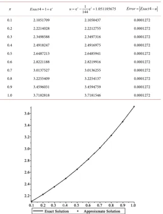
Table 4. Numerical results and exact solution of Nonlinear Fredholm integral equation of the second kind for example 4.
4
Error Exact= −u
2
1
e e 1.051185675
144
x
u= − +
4 1 ex
Exact = + x
0.0001272 2.1050437
2.1051709 0.1
0.0001272 2.2212755
2.2214028 0.2
0.0001272 2.3497316
2.3498588 0.3
0.0001272 2.4916975
2.4918247 0.4
0.0001272 2.6485941
2.6487213 0.5
0.0001272 2.8219916
2.8221188 0.6
0.0001272 3.0136255
3.0137527 0.7
0.0001272 3.2254137
3.2255409 0.8
0.0001272 3.4594759
3.4596031 0.9
0.0001272 3.7181546
3.7182818 1.0
Figure 4. The exact and approximate solutions result of Nonlinear Fredholm integral eq-uation of the Second kind.
Example 5. Consider the nonlinear Fredholm integral equation of the second kind
( )
( )
2(
2( )
)
0
1
sin 1 d ,
64 48
u x = x −π +
∫
πt +u t t (7)with the exact solution u x
( )
=sin( )
x .Example 6. Consider the nonlinear Fredholm integral equation of the second kind
( )
( )
(
2( )
)
0
5 1
sin 1 1 d
16 12 48
u x = x + − + + πt u u t+ t
π π
DOI: 10.4236/apm.2019.910040 838 Advances in Pure Mathematics
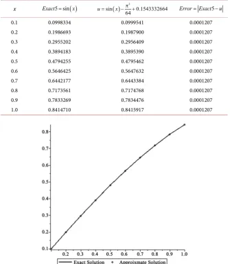
Table 5. Numerical results and exact solution of Nonlinear Fredholm integral equation of the second kind for example 5.
5
Error Exact= −u
( ) 2 0.
sin 1543332 6
4 6
6 4
u= x −π +
( )
5 sin
Exact = x
x 0.0001207 0.0999541 0.0998334 0.1 0.0001207 0.1987900 0.1986693 0.2 0.0001207 0.2956409 0.2955202 0.3 0.0001207 0.3895390 0.3894183 0.4 0.0001207 0.4795462 0.4794255 0.5 0.0001207 0.5647632 0.5646425 0.6 0.0001207 0.6443384 0.6442177 0.7 0.0001207 0.7174768 0.7173561 0.8 0.0001207 0.7834476 0.7833269 0.9 0.0001207 0.8415917 0.8414710 1.0
[image:7.595.207.539.562.728.2]Figure 5. The exact and approximate solutions result of Nonlinear Fredholm integral eq-uation of the second kind.
Table 6. Numerical results and exact solution of Nonlinear Fredholm integral equation of the second kind for example 6.
6
Error Exact= −u
( )
sin 0.9808838911
u= x +
( )
6 1 sin
Exact = + x
DOI: 10.4236/apm.2019.910040 839 Advances in Pure Mathematics with the exact solution u x
( )
= +1 sin( )
x .Example 7. Consider the nonlinear Fredholm integral equation of the second kind
( )
( )
2(
2( )
)
0
7 5 1
cos d ,
6 144 36
u x = x + − π +
∫
πt u u t+ t (9) [image:8.595.242.513.134.435.2]with the exact solution u x
( )
= +1 cos( )
xFigure 6. The exact and approximate solutions result of Nonlinear Fredholm integral eq-uation of the Second kind.
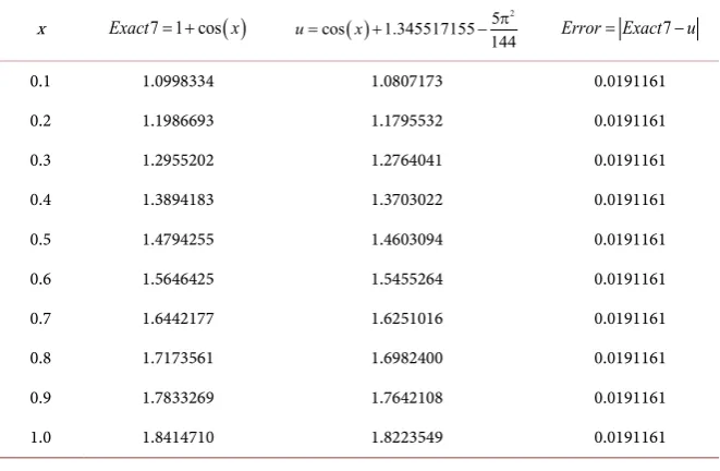
Table 7. Numerical results and exact solution of Nonlinear Fredholm integral equation of the second kind for example 7.
7
Error Exact= −u
( ) 5 2
cos 1.345517155 144
u= x + − π
( )
7 1 cos
Exact = + x
x
0.0191161 1.0807173
1.0998334 0.1
0.0191161 1.1795532
1.1986693 0.2
0.0191161 1.2764041
1.2955202 0.3
0.0191161 1.3703022
1.3894183 0.4
0.0191161 1.4603094
1.4794255 0.5
0.0191161 1.5455264
1.5646425 0.6
0.0191161 1.6251016
1.6442177 0.7
0.0191161 1.6982400
1.7173561 0.8
0.0191161 1.7642108
1.7833269 0.9
0.0191161 1.8223549
[image:8.595.208.539.512.728.2]DOI: 10.4236/apm.2019.910040 840 Advances in Pure Mathematics
Figure 7. The exact and approximate solutions result of Nonlinear Fredholm integral equation of the Second kind.
4. Conclusion
In the paper, a successive approximations method is presented for solving the nonlinear Fredholm integral equation of the second kind using Maple18. The benefit of our method lies in the fact that, for some nonlinear problems, our method is still convergent as illustrated by figures and tables showing match the right accuracy, which shows the exact solution with the approximate solution is largely identical and noticeable Tables 1-7 represent the exact and numerical results of the examples in this article. Figures 1-7 readily show the comparison of exact solution and approximate solution.We can see from the figures that the approximate solution is very applicable to the exact solution and application is displayed through some examples. Numerical results show that the accuracy of the solutions obtained is good.
Acknowledgements
This project was funded by the Deanship of Scientific Research (DSR), King Abdulaziz University. The author, therefore, acknowledges with thanks to DSR technical and financial support.
Conflicts of Interest
The author declares no conflicts of interest regarding the publication of this pa-per.
References
DOI: 10.4236/apm.2019.910040 841 Advances in Pure Mathematics
https://doi.org/10.1016/S0045-7825(99)00018-3
[2] He, J.H. (2000) A Coupling Method of a Homotopy Technique and a Perturbation Technique. International Journal of Non-Linear Mechanics, 35, 37-43.
https://doi.org/10.1016/S0020-7462(98)00085-7
[3] He, J.H. (2003) Homotopy Perturbation Method: A New Non-Linear Analytical Technique. Applied Mathematics and Computation, 135, 73-79.
https://doi.org/10.1016/S0096-3003(01)00312-5
[4] He, J.H. (2004) Asymptotology by Homotopy Perturbation Method. Applied Ma-thematics and Computation, 156, 591-596.
https://doi.org/10.1016/j.amc.2003.08.011
[5] He, J.H. (2005) Application of Homotopy Perturbation Method to Nonlinear Wave Equations. Chaos, Solitons and Fractals, 26, 695-700.
https://doi.org/10.1016/j.chaos.2005.03.006
[6] He, J.H. (2006) Homotopy Perturbation Method for Solving Boundary Value Prob-lems. Physics Letters A, 350, 87-88.https://doi.org/10.1016/j.physleta.2005.10.005
[7] He, J.H. (2006) New Interpretation of Homotopy Perturbation Method. Interna-tional Journal of Modern Physics B, 18, 2561-2568.
https://doi.org/10.1142/S0217979206034819
[8] Balakumar, V. and Murugesan, K. (2013) Numerical Solution of Systems of Linear Volterra Integral Equations Using Block-Pulse Functions, Malaya. Journal of Ma-thematic, 1, 77-84.
[9] Burden, R.L. and Douglas Faires, J. (2005) Numerical Analysis. 8th Edition, Thom-son Brooks/Cole, Belmont.
[10] Burton, T.A. (2005) Volterra Integral and Differential Equations. 2nd Edition, Ma-thematics in Science & Engineering, Elsevier, Amsterdam, 202.
[11] Berenguer, M.I., Gamez, D., Garralda-Guillem, A.I., Ruiz Galan, M. and Serrano Perez, M.C. (2011) Biorthogonal Systems for Solving Volterra Integral Equation Systems of the Second Kind. Journal of Computational and Applied Mathematics, 235, 1875-1883.https://doi.org/10.1016/j.cam.2010.07.011
[12] Biazar, J. and Eslami, M. (2011) Modified HPM for Solving Systems of Volterra Integral Equation of the Second Kind. Journal of King Saud University-Science, 23, 35-39.https://doi.org/10.1016/j.jksus.2010.06.004
[13] Linz, P. (1985) Analytical and Numerical Methods for Volterra Equations. Studies in Applied Mathematics 7, SIAM, Philadelphia.
https://doi.org/10.1137/1.9781611970852
[14] Mirzaee, F. (2010) Numerical Computational Solution of the Linear Volterra Integral Equations System via Rationalized Hear Functions. Journal of King Saud University-Science, 4, 265-268.https://doi.org/10.1016/j.jksus.2010.05.010
[15] Wazwaz, A.M. (2011) Linear and Nonlinear Integral Equation: Methods and Ap-plications. Springer, Berlin.https://doi.org/10.1007/978-3-642-21449-3
[16] Effati, S. and Noori Skandari, M.H. (2012) Optimal Control Approach for Solving Linear Volterra Integral Equations. International Journal of Intelligent Systems and Applications, 4, 40-46.https://doi.org/10.5815/ijisa.2012.04.06
[17] Maturi, D.A. (2014) Numerical Solution of System of Two Nonlinear Volterra Integral Equations. International Journal of Computers & Technology, 12, 3967-3975.https://doi.org/10.24297/ijct.v12i10.2989
DOI: 10.4236/apm.2019.910040 842 Advances in Pure Mathematics Advances in Mathematics, 8, 1540-1553.
[19] Maturi, D.A. (2014) Adomian Decomposition Method of Fredholm Integral Equa-tion of the Second Kind Using Maple. Journal of Advances in Mathematics, 9, 1868-1875.
[20] Maturi, D.A. (2014) Application of Adomian Decomposition Method for Solving of Fredholm Integral Equation of the Second Kind. European Journal of Science and Engineering, 9, 1-9.
[21] Sorkun, H.H. and Yalcinbas, S. (2010) Approximate Solutions of Linear Volterra Integral Equation Systems with Variable Coefficients. Applied Mathematical Mod-eling, 34, 3451-3464.https://doi.org/10.1016/j.apm.2010.02.034
[22] Maturi, D.A. and Malaikah, H. (2018) Numerical Solution of System of Three Non-linear Volterra Integral Equation Using Implicit Trapezoidal. Journal of Mathemat-ics Research, 10, 44.https://doi.org/10.5539/jmr.v10n1p44
[23] Ostvoar, A.A. and Hasina, M. (1999) Solving nth-Order Integro-Differential Equa-tions Using the Combined Laplace Transfor-Successive ApproximaEqua-tions Method. Communications on Advanced Computational Science with Applications, 178, 257-262.
[24] Khan, F., Mustafa, G., Omar, M. and Komal, H. (2017) Numerical Approach Based on Bernstein Polynomials for Solving Mixed Volterra-Fredholm Integral Equations. AIP Advances, 7, 125-123.https://doi.org/10.1063/1.5008818
[25] Huanga, G.X. and Yin, F. (2011) An Inverse Eigenproblem and an Associated Ap-proximation Problem for Generalized Reflexive and Anti-Reflexive Matrices. Jour-nal of ComputatioJour-nal and Applied Mathematics, 235, 2888-2895.
https://doi.org/10.1016/j.cam.2010.12.016
[26] Behiry, S.H., Abd-Elmonem, R.A. and Gomaa, A.M. (2010) Discrete Adomian De-composition Solution of Nonlinear Fredholm Integral Equation. Ain Shams Engi-neering Journal, 1, 97-101.https://doi.org/10.1016/j.asej.2010.09.009
[27] Biazar, J., Ghanbari, B. and Porshokouhi, M.G. (2011) He’s Homotopy Perturbation Method: A Strongly Promising Method for Solving Non-Linear Systems of the Mixed Volterra-Fredholm Integral Equations. Computers and Mathematics with Applications, 61, 1016-1023.https://doi.org/10.1016/j.camwa.2010.12.051
[28] Ayati, Z. and Biazar, J. (2015) On the Convergence of Homotopy Perturbation Me-thod. Journal of the Egyptian Mathematical Society, 23, 424-428.
https://doi.org/10.1016/j.joems.2014.06.015
[29] Biazar, J. and Ghanbari, B. (2012) The Homotopy Perturbation Method for Solving Neutral Functional-Differential Equations with Proportional Delays. Journal of King Saud University-Science, 24, 33-37.https://doi.org/10.1016/j.jksus.2010.07.026
[30] Wu, G.C., Baleanu, D. and Deng, Z.G. (2015) Variational Iteration Method as a Kernel Constructive Technique. Applied Mathematical Modelling, 39, 4378-4384. https://doi.org/10.1016/j.apm.2014.12.032
[31] Dong, C., Chen, Z. and Jiang, W. (2013) A Modified Homotopy Perturbation Me-thod for Solving the Nonlinear Mixed Volterra-Fredholm Integral Equation. Jour-nal of ComputatioJour-nal and Applied Mathematics, 239, 359-366.
https://doi.org/10.1016/j.cam.2012.09.003
[32] Turkyilmazoglu, M. (2010) A Note on the Homotopy Analysis Method. Applied Mathematics Letters, 23, 1226-1230.https://doi.org/10.1016/j.aml.2010.06.003
DOI: 10.4236/apm.2019.910040 843 Advances in Pure Mathematics of the Association of Arab Universities for Basic and Applied Sciences, 24, 149-155. https://doi.org/10.1016/j.jaubas.2016.08.002
[34] Eldeberky, Y. (2011) Modeling Spectra of Breaking Waves Propagating Overa Beach. Ain Shams Engineering Journal, 2, 71-77.
https://doi.org/10.1016/j.asej.2011.07.002
[35] Daoud, Y. and Khidir, A.A. (2018) Modified Adomian Decomposition Method for Solving the Problem of Boundary Layer Convective Heat Transfer. Propulsion and Power Research, 7, 231-237.https://doi.org/10.1016/j.jppr.2018.05.005