go.warwick.ac.uk/lib-publications
Original citation:
Hine, Nicholas, Dziedzic, Jacek, Haynes, Peter D. and Skylaris, Chris-Kriton. (2011)
Electrostatic interactions in finite systems treated with periodic boundary conditions :
application to linear-scaling density functional theory. Journal of Chemical Physics, 135 (20).
204103.
Permanent WRAP URL:
http://wrap.warwick.ac.uk/71498
Copyright and reuse:
The Warwick Research Archive Portal (WRAP) makes this work by researchers of the
University of Warwick available open access under the following conditions. Copyright ©
and all moral rights to the version of the paper presented here belong to the individual
author(s) and/or other copyright owners. To the extent reasonable and practicable the
material made available in WRAP has been checked for eligibility before being made
available.
Copies of full items can be used for personal research or study, educational, or not-for profit
purposes without prior permission or charge. Provided that the authors, title and full
bibliographic details are credited, a hyperlink and/or URL is given for the original metadata
page and the content is not changed in any way.
Publisher’s statement:
This article may be downloaded for personal use only. Any other use requires prior
permission of the author and AIP Publishing.
The following article appeared in Journal of Chemical Physics and may be found at
http://scitation.aip.org/content/aip/journal/jcp/135/20/10.1063/1.3662863
A note on versions:
The version presented here may differ from the published version or, version of record, if
you wish to cite this item you are advised to consult the publisher’s version.
Electrostatic Interactions in Finite Systems treated with Periodic Boundary Conditions: Application to Linear-Scaling Density Functional Theory
Nicholas D. M. Hine,1,a)Jacek Dziedzic,2Peter D. Haynes,1and Chris-Kriton Skylaris2
1)Department of Physics and Department of Materials, Imperial College London, Exhibition Road,
London SW7 2AZ, UK.
2)School of Chemistry, University of Southampton, Highfield, Southampton SO17 1BJ,
UK.b)
(Dated: November 10, 2011)
We present a comparison of methods for treating the electrostatic interactions of finite, isolated systems within periodic boundary conditions (PBCs), within Density Functional Theory (DFT), with particular emphasis on linear-scaling (LS) DFT. Often, PBCs are not physically realistic but are an unavoidable consequence of the choice of basis set and the efficacy of using Fourier transforms to compute the Hartree potential. In such cases the effects of PBCs on the calculations need to be avoided, so that the results obtained represent the open rather than the periodic boundary. The very large systems encountered in LS-DFT make the demands of the supercell approximation for isolated systems more difficult to manage, and we show cases where the open boundary (infinite cell) result cannot be obtained from extrapolation of calculations from periodic cells of increasing size. We discuss, implement and test three very different approaches for overcoming or circumventing the effects of PBCs: truncation of the Coulomb interaction combined with padding of the simulation cell, approaches based on the minimum image convention, and the explicit use of Open Boundary Conditions (OBCs). We have implemented these approaches in the ONETEP LS-DFT program and applied them to a range of systems, including a polar nanorod and a protein. We compare their accuracy, complexity, and rate of convergence with simulation cell size. We demonstrate that corrective approaches within PBCs can achieve the OBC result more efficiently and accurately than pure OBC approaches.
I. INTRODUCTION
Density Functional Theory (DFT)1,2is widely and
rou-tinely used for computational electronic structure simu-lations due to its favorable balance of speed and accu-racy. However, making DFT simulations scale well to the numbers of atoms required to study large complex systems such as proteins and nanostructures presents sig-nificant challenges. Various linear-scaling approaches to DFT have emerged over the last two decades to meet this challenge3–17. Several of these methods use basis
sets which are related to plane waves and require peri-odic boundary conditions (PBCs). The plane-wave pseu-dopotential approach has been developed with crystalline systems in mind, and as these are genuinely periodic, the treatment of electrostatics in the framework of PBCs was a natural choice with significant advantages. In re-ciprocal space, the Hartree interaction is diagonal, so the Hartree potential and energy are easily obtained us-ing Fast Fourier Transforms (FFTs). Furthermore, the plane-wave basis set is systematic in the sense that it provides a uniform description of space and can be im-proved by increasing the value of one parameter.
However, the increasing use of linear-scaling DFT (LS-DFT) in large systems highlights long-standing issues in electronic structure methods relating to the treatment of electrostatic interactions, i.e. the long-ranged parts of
a)Electronic mail: [email protected]
b)Also at: Faculty of Technical Physics and Applied Mathematics, Gdansk University of Technology, Poland.
the Coulomb interaction between electron density and electron density (‘Hartree’ terms), electron density and ion cores, and between ion cores, under PBCs.
Bulk systems can be genuinely periodic and then the influence of periodic replicas is desired; however, to al-low simulation of finite, isolated systems within PBCs, the supercell approximation is widely used18–20. This
involves the replacement of a genuinely isolated system with a lattice of periodic replicas, with vacuum ‘padding’ surrounding the system to reduce the influence of peri-odic replicas on each other. While this is a reasonable approach, it introduces finite size errors whereby the to-tal energy varies with supercell size.
extrapo-lating to infinite supercell size. This issue is exacerbated as the isolated molecules and their dipole moments be-come larger.
To address this problem, a large range of techniques that aim to either reduce or eliminate the effects of the PBCs on the electrostatics of grid-based electronic struc-ture calculations have been developed over the recent years21–37. These include methods which attempt to
formulate ana posteriori correction term to add to the
energy22,23,25on the basis of a multipole expansion of the
localised charge, having first inserted a uniform periodic background to counter any monopole charge38; methods
which formulate a more complex form of ‘counter-charge’ which counteracts the periodic interactions26,28,29,36,37,
and methods that modify the form of the interaction in real or reciprocal space in order to avoid the existence of periodic interactions in the first place24,27,30–32,35.
In this paper, we examine, implement and compare three different approaches fulfilling these criteria: trun-cation of the Coulomb interaction in real space, referred to here as ‘Cutoff Coulomb’ (CC)24,31; the approaches
of Martyna and Tuckerman (MT) and Genovese et al.,
which replace the periodic Coulomb interaction with a Minimum Image Convention (MIC) approach to the Coulomb potential27; and the replacement of PBCs with
Open Boundary Conditions (OBCs) using a multigrid ap-proach to the Poisson equation39–41. These methods are
implemented and tested on a range of systems represent-ing typical cases with challengrepresent-ing electrostatic properties. We compare their accuracy, convergence properties, com-plexity and computational overhead, and summarise the advantages and disadvantages of each.
Throughout this work, we employ linear-scaling DFT with the ONETEP code42, and while our findings will
be applicable to all electronic structure methods, linear-scaling or otherwise, we focus in particular on the chal-lenges encountered applying these methods to large, com-plex systems. System size can be measured either by the number of atomsN included in the simulation, or by the volumeV of the simulation cell — the latter being partic-ularly relevant in the case of isolated systems. ONETEP combines linear-scaling computational effort, in that the total computational time for a simulation of N atoms can be made to scale as O(N), with near-independence of the computational effort on the amount of vacuum padding (i.e.nearly independent of V at fixed N), and systematic control of the accuracy with respect to the basis, akin to that of plane-wave DFT. The requirements on any method used to treat electrostatic interactions are therefore that it must have systematically control-lable accuracy, must not impose too high a computational overhead, and must have low-order scaling with N and V.
II. ELECTROSTATICS IN
LINEAR-SCALING DENSITY FUNCTIONAL THEORY
The calculations in this work are performed with the ONETEP Linear-Scaling DFT approach. Like most linear-scaling approaches to DFT, ONETEP uses the density matrix rather than eigenstates of the Hamil-tonian, representing the single-electron density matrix ρ(r,r′)in terms of nonorthogonal localised orbitalsφα(r)
and a ‘density kernel’Kαβas
ρ(r,r′) =φα(r)Kαβφβ(r′). (1)
The Einstein convention of summation over repeated Greek indices will be employed throughout. Using the density matrix, the electron density n(r) can be found
from
n(r) =ρ(r,r) =φα(r)Kαβφβ(r). (2)
Where ONETEP differs from most linear-scaling approaches is that the local orbitals, referred to as Nonorthogonal Generalised Wannier Functions (NGWFs)43, are themselves expressed in a systematic
underyling basis of periodic-sinc functions (psincs), and are therefore systematically convergeable. This is achieved by a double-loop optimisation44 of both the
coefficients Ciα of the psinc functions Di(r) describing each NGWF and the elements of the density kernelKαβ:
ET= min {Ciα}
L({Ciα}), (3)
whereLrepresents optimisation with respect to the den-sity kernel, a generalisation of the occupancies, through:
L({Ciα}) = min {Kαβ}E({K
αβ};{C
iα}). (4)
This results in a method with controllable accuracy and systematic convergence of total energies and forces with respect to basis size, equivalent to the plane-wave ap-proach45,46, in systems of tens of thousands of atoms47,48.
Convergence is controlled by varying the spacing of the psinc grid, in a manner equivalent to varying a plane-wave cutoff, described by a cutoff energy Ecut, and by
varying the cutoff radii of the spherically-truncated NG-WFs, described by a sphere radiusRφ. To achieve true asymptotically linear scaling behaviour, it is also neces-sary to truncate the range of the density kernelKαβ so that elements for NGWFs centred on distant atoms for which |Rα−Rβ| > RK are set to zero. However, this
latter form of truncation is only necessary in very large systems and will not be considered in this work.
the classical density-density interaction; the local pseu-dopotential term, Elocps[n], which is the interaction of the electron density with the long-ranged part of the po-tential resulting from the ion cores; and the interaction between the ion cores,Eion−ion. It should be noted that during the optimisation of the kernel and NGWF coeffi-cients Kαβ and C
iα, the full interacting energy is min-imised by conjugate gradients process, meaning that no mixing of densities is required at any point. The prob-lem, then, becomes one simply of evaluating EH[n] and VH[n](r)for a given densityn(r)(which always integrates fo the number of electronsNe).
To be absolutely clear on the formalism involved, we will briefly re-visit the standard approach, making careful distinctions on how the expressions and their meaning vary under PBCs and under OBCs, where the potentials tend to zero at infinity. In both cases, the Hartree energy can be obtained as EH = 12
´
n(r)VH(r)dr, where the
Hartree potentialVH(r)resulting from a densityn(r), is formally obtained by solving the Poisson equation:
∇2VH(r) =−4πn(r). (5)
Note that we are working in atomic units, for which 1/ε0 = 4π. This can in general be solved through the use of the corresponding Green function G(r,r′) = −1/4π|r−r′|, producing
VH(r) =−
ˆ
all space
n(r′)
|r−r′|dr
′.
This result builds in the OBC definition that the poten-tial goes to zero at infinity, and cannot be used directly to evaluateEHor VH(r)under PBCs as the integral has infinite value at allrfor periodicn(r′).
When PBCs are used Eq. (5) is only valid for charge distributions of zero charge per simulation cell. If the total charge on one cellq=´
Ωn(r)dris non-zero, Eq. (5) is modified to the following form:
∇2VH(r) =−4π(n(r)−q/Ω), (6)
where Ω is the volume of the simulation cell. This is equivalent to the insertion of a uniform background charge density of equal and opposite charge to n(r) so
that the total charge is zero. A periodic density will result in a periodic potential and in this case we can re-write both sides of Eq. (6) in terms of their discrete Fourier transforms and rearrange to obtain
˜
VH(G) = 4π
ΩG2(˜n(G)−qδG,0) . (7) Note that Eq. (7) makes clear the utility of a recipro-cal space approach to recipro-calculating V˜H(G), even outside
of a genuinely periodic situation: the Coulomb interac-tion is diagonal in reciprocal space, so V˜H(G) can be
obtained trivially fromn˜(G). After obtaining VH(r) by
an inverse FFT, the integralEH= 12
´
Ωn(r)VH(r)drcan be performed only over one simulation cell to obtain the Hartree energy per simulation cell.
Sim. cell
Sim. cell Sim. cell
Sim. cell Sim. cell Sim. cell
periodically repeated functions
sum of periodically repeated functions
resulting periodic function in simulation cell
single function single function made periodic with M.I.C.
[image:4.595.332.537.74.229.2]resulting periodic function in simulation cell
Figure 1. Different ways of making a function obey periodic boundary conditions inside a simulation cell, demonstrated for a Gaussian function. Top panel: The Fourier transform approach. The resulting function is the same as the one that would be obtained by a superposition (sum) of periodically re-peated Gaussians. Bottom panel: The Minimum Image Con-vention (MIC) approach: the resulting function is the same as the one that would be obtained by having a single Gaussian in the simulation cell and making it periodic by applying the MIC.
In PBCs the potential is, by definition, the result of contributions from not just then(r)of the home
simula-tion cell but also from the densities of an infinite number of periodic replicas of that cell. A periodic function that can be constructed in this way is demonstrated with the example at the top panel of Figure 1. As we have already mentioned, the potential and the electrostatic energy di-verge for non-zero total charge in the simulation cell (or equivalently whenn˜(G= 0) is nonzero). To avoid this
divergence one must setn˜(G= 0)to zero for each
com-ponent making up total charge density (including the ion charges) to ensure that the result is finite. Having made this choice however, one alters the problem being studied as the potentialVH(r)obtained is that resulting not just from the infinite periodic array ofn(r), but also from a
neutralising charge distribution, which is usually taken to be a uniform background charge over the whole cell.
The same arguments apply to the other electrostatic terms, by replacing the electron density n(r) with the
charge density of the ions, in the form of a collection of point charges. For an isolated system, the energy of interaction of the ions is of course simply
Eion-ion= 1 2
X
I, J6=I
ZIZJ
|RI−RJ| , (8)
while under PBCs, in the presence of the neutralising background, the energy of interaction per unit cell is most commonly calculated using the Ewald technique49.
electronic structure calculation. Therefore, it should be immediately clear that noa posteriori approach to
cor-recting total energies obtained from a simulation under PBCs can be completely successful in providing total en-ergies that match those of an isolated system as even after the “removal” of the periodicity the density will remain distorted to what it was in the periodic calculation. Here we examine three approaches that are applied within the self-consistent procedure and therefore are able to correct not only the energy but also the potential.
III. CUTOFF COULOMB INTERACTIONS
One way to avoid the effects of PBCs which are intrin-sic to the discrete Fourier representation of the Coulomb potential is to use a modified form for the Coulomb po-tential. One such possibility is the use of a "cutoff" form of the Coulomb interaction. This allows the usual Fourier transform-based approach to be used, including a nomi-nally periodic simulation cell, but truncates the Coulomb potential so that it is confined within the primary simula-tion cell. The approach has been applied by several pre-vious works24,31and is implemented in several codes50,51.
The essence of the cutoff Coulomb approach is that the periodic, background-neutralised Coulomb potential VEw(r) is replaced with the bare Coulomb interaction, truncated so as to prevent any part of the simulation cell feeling the potential from any neighbouring copy. This removes the need for the canceling background, even though the charge density is periodically repeated. Some new complications arise however as the cutoff Coulomb potential needs to be generated in reciprocal space.
To retain the simplicity of having an interaction that is diagonal in reciprocal space, but still avoid the influence of periodic replicas, one can use the following form for the Coulomb potential
VCC(r−r′) =
( 1
|r−r′| r−r′ ∈ R1
0 r−r′ ∈ R/ 1 . (9)
R1is a region of a size and shape chosen such that when centered at any point rat which VH(r)is required (this
may be anywhere inside the main simulation cell, or it may just be anywhere where the density is nonzero),R1 encloses all r′ for which n(r+r′) 6= 0. The Hartree
potential is now obtained as the convolution of the cut-off Coulomb operator and the density
VH(r) =
ˆ
Ω
n(r′)VCC(r−r′) dr′ . (10)
The simplest shape for R1 is a sphere of radius Rc, for whichVCCsphere(r) = Θ(|r| −Rc)/|r|whereΘis the
Heavi-side step function. In this case, the Fourier transform of the interaction is well-known:
˜
VCCsphere(G) = 4π(1−cos(GRc))
[image:5.595.366.512.49.202.2]ΩG2 . (11)
Figure 2. Illustration of the cell sizesLcell, Lpad and cutoff
radiusRcrequired for the spherical cutoff Coulomb approach.
Rc must be at least as large as the largest distance between
any two non-zero charges in the system (this is trivially
sat-isfied ifRc≥
√
3Lcell). In order for the periodic densities not
to impinge on each other,Lpad≥(Lmol+Rc) must be
sat-isfied, whereLmol is the extent of the system (again, defined
as maximum distance between two non-zero charges) in any Cartesian direction.
As this function does not have a singularity atG= 0the
Hartree potential is obtained in reciprocal space as its product with˜n(G)as in Eq. (7) but without theqterm
as there is no longer the need to include a uniform back-ground charge. A spherical cutoff removes the periodicity in all three spatial dimensions. If periodicity is retained in one or two dimensions there are corresponding forms for V˜CC(G) to account for these wire (1D periodicity)
and slab (2D periodicity) geometries. A comprehensive study was made by Rozziet. al.31 describing the terms
of the cutoff Coulomb interaction for each geometry. In a practical calculation, the electron densityn(r) on a
real space grid over the original simulation cell is trans-ferred to a grid for a larger ‘padded’ cell of size Lpad and padded with zeros, then Fourier transformed to give ˜
npad(G). The terms of V˜CC(G) are calculated for this reciprocal space grid in advance and stored, and are used to multiply the Fourier components n˜pad(G) whenever the Hartree potential is required. Reverse Fourier trans-forming these components givesVH,pad(r)from which the values ofVH(r)on the original cell are extracted.
The corresponding cut-off form of the Coulomb inter-action must also be used in place of the long-ranged Coulombic tail of the ion cores in the local pseudopo-tentialVlocps(r). To achieve this, V˜locps(G)is calculated over the whole padded grid, replacing the 4π
ΩG2Zionterm byV˜CC(G)Zion for the relevant form of cutoff Coulomb
interaction. This is then transformed to real space by Fourier transform and extracted to the standard grid to give the required form of Vlocps(r). Similarly, the peri-odic Coulomb and Ewald terms in the calculation of the forces acting on the ion cores are replaced by their cutoff Coulomb forms.
an SCF calculation compared to the traditional PBC Fourier transform Coulomb approach consists of three parts: transfer of the calculated density from the original grid to a larger, padded grid, calculation of the forward and backwards Fast Fourier Transforms required for the Hartree potential on the larger grid, and extraction of the calculated potential from the larger grid back to the original one. The first and last of these are in general comparatively trivial and take very little time. Perform-ing the FFT on the larger grid often incurs a considerable slowdown relative to performing it on the original grid, but nevertheless, generally speaking, this part of the cal-culation takes a almost negligible fraction of the total computational time for large enough systems.
When simulating an isolated object such as a nanocrys-tal or nanotube with a high aspect ratio, the geometry of the system requires that we use a simulation cell that is very long in one dimension (thexdirection here) and comparatively small in the other two (yandz). Perform-ing cutoff Coulomb calculations with a spherical cutoff would rapidly become impractical as the length of the system is increased, since for a sphere geometry, we would be required to embed the original cell in a padded cell with all the side lengthsLx, Ly, Lz> Rc. In such cases, we need to define a geometry for the cutoff Coulomb in-teraction such that the cutoff range can be very long in one direction and shorter in the other two. One obvious choice for a long, thin system is to cut off the Coulomb interaction on the surface of a cylinder. In this case, the integrals required to evaluate the coefficients are not an-alytically solvable but can be put in a form amenable to numerical evaluation. Appendix A gives details on the evaluation of the Fourier coefficients of the interaction for a cylindrical cutoff. With an efficient system for eval-uating the termsVCC(G)numerically, the interaction can be calculated rapidly in advance and reused, and simu-lations of isolated high aspect ratio systems can proceed within cells of feasible size.
IV. MINIMUM IMAGE CONVENTION
An alternative technique for avoiding periodic inter-actions is the class of approaches which includes those of Martyna-Tuckerman27 and Genovese et al32,35. The
essence of these, which we will call Minimum Image Convention (MIC) approaches is that the form of the Coulomb operator is modified in a way that is still peri-odic (as this is unavoidable if standard FFTs are to be used) but which nevertheless removes contributions from neighbouring cells.
To see how this is achieved, we consider first the Fourier transform of a functionf(r), defined as
˜
f(G) = ˆ
all spacee −iG·r
f(r)dr. (12)
In PBCs, a discrete set of wave vectors G are used to
expand functions in Fourier space. These wavevectors
are chosen by the requirement that they need to be com-mensurate with the simulation cell. Therefore, given the expression forf˜(G), the real space representation of the
functionf(r)under PBCs is the following:
fper(r) =
X
G∈cell ˜
f(G)eiG·r . (13)
This is an exact result and shows that the Fourier rep-resentation of f(r) in the simulation cell is a periodic
function fper(r) with the periodicity of the simulation cell. It is important to notice is that this function is constructed as a superposition of periodically repeated functionsf(r), one in each cell. This is demonstrated for
the example of a Gaussian function in the top panel of Figure 1, where its resulting periodic form in one simu-lation cell is provided, as it would be generated in real space as a Fourier expansion by Eq. (13). This result implies that periodic interactions are unavoidable if the potential is constructed by approaches based on Fourier transforms in the standard simulation cell, as PBCs are implicit in such procedures. However, MIC approaches are designed to avoid the part of the Coulomb interaction which produces this undesired long-ranged interaction.
We have implemented the Martyna-Tuckerman approach27, in which the Fourier method is used to
construct not the periodic function fper(r) but the periodic functionfMIC(r) which results by making f(r) periodic over a single simulation cell using the MIC49.
A similar approach can also be employed in Quantum Monte Carlo calculations, via the “Model Periodic Coulomb” approach52,53. The distinction between
fper(r) and fMIC(r) is clarified in Figure 1 where the bottom panel demonstrates the construction of fMIC(r) for the example of a Gaussian function.
To work with this formalism we need to determine the Fourier transformf(G)that will produce the desired
fMIC(r)
fMIC(r) =
X
G cell
f(G)eiG·r . (14)
As this method is intended for dealing with the Coulomb potential, from now on we will fix the functionf(r)to be
equal toφ(r) = 1/r so that we can focus on particular
issues that arise in this case. In determining the form ofφ(G) we need to deal with the extra complication of
the singularity of the potential atr → 0 (short range)
and at G→ 0 (long range). The Coulomb potential is
partitioned as
1
r =
erf(αr)
r +
erfc(αr)
Fourier transform is expressed as
φ(G) =φlong(G) + ˜φshort(G) (16)
= [φlong(G)−φ˜long(G)] + [ ˜φlong(G) + ˜φshort(G)]
= ˆφscreen(G) + ˜φ(G) , (17)
where the explicit expression for φ˜short(G)is
˜
φshort(G) = 4π G2
1−exp
−G
2
4α2
. (18)
Eq. (16) can also be further expanded to the form shown in Eq. (17) which demonstrates that the MT for-malism is equivalent to augmentingφ˜(G)with a
“screen-ing potential” φˆscreen(G) which cuts off the interactions
from the periodic images of the simulation cell. In prac-tice, we computeφ(G)according to Eq. (16) and we
dis-tinguish two cases: G6=0 and G=0, which must be
treated separately.
The functionφlong(G)forG6=0is obtained as
φlong(G) =
ˆ
Ω
e−iG·rerf(αr)
r dr, (19)
where the above integral is computed as a sum over the simulation cell grid points as this is an exact expression for the wavevectorsGwhich are commensurate with the
simulation cell. The above expression is the desired one as the termerf(αr)/rdoes not contain contributions from periodic images. It also does not contain a singularity at r= 0so the evaluation of this integral poses no difficul-ties. The complete expression forφ(G)is obtained as the
sum of the terms Eq. (18) and Eq. (19).
To find theG=0term, we need to consider the limit
of Eq. (18) asGgoes to zero
lim G→0
˜
φshort(G) =
= lim G→0
4π G2
1−
1− G
2
4α2 + G4
8α4 +· · ·
= π
α2 (20)
and taking this into account, Eq. (16) becomes
φ(0) =φlong(0) + ˜φshort(0)
=
ˆ
Ω
erf(αr)
r dr+ π
α2 , (21)
where the integral in the above expression is again eval-uated as a sum over the simulation cell grid points as the integrand does not contain a singularity atr= 0.
In order to use the MT potential in practical calcu-lations, we need to ensure that appropriate conditions are obeyed as regards the relative sizes of the simulated molecule and the simulation cell. From the example in the bottom panel of Figure 1 we can see that the length that a simulation cell can have in any direction needs to be at least twice the length of the molecule being simu-lated. In the opposite case unphysical interactions will
be introduced as some charges on the molecule will be experiencing the Coulomb potential from other parts of the molecule (as they should) while other charges will ex-perience the potential from a periodic image (which they should not).
In our implementation the Hartree potential is gener-ated in reciprocal space from the electronic density as a product with the Fourier transform of MT potential φ(G)
VH(G) =φ(G)˜n(G). (22)
In a similar way, the local pseudopotential is obtained in reciprocal space as a sum of short and long range terms
Vlocps(G) =Vlocps,short(G) +Vlocps,long(G) . (23)
For an ion with charge −Z, (following the established electronic structure theory convention of taking the ionic potential as negative), the periodic Coulomb component is subtracted from the pseudopotential to obtain its short range part
Vlocps,short(G) = ˜Vlocps(G) +Zφ˜(G) (24)
and the long range part is obtained as the MIC Coulomb interaction
Vlocps,long(G) =−Zφlong(G). (25)
Finally the core-core interaction energy is obtained as a Coulombic sum between point charge interactions in the simulation cell according to Eq. (8).
Genovese et al.32,35 proposed an approach that is
rather similar in principle but in practice has some dif-ferent properties. They described a wavelet-based ap-proach to calculating the MIC Coulomb interaction. The charge density is expanded using interpolating scaling functions54 of order m (typically m = 14). This
guar-antees that when a known continuous charge density is represented, the first m moments are preserved. Al-though most practical methods do not attempt to rep-resent given continuous charge densities, this approach is useful when using pseudopotentials of the form proposed by Goedeckeret al.55. The representation of the Coulomb
operator is made separable by employing an expansion in terms of Gaussians56. The resulting one-dimensional
V. OPEN BOUNDARY CONDITIONS
The final possibility we will consider is to change not the form of the interactions, but that of the bound-ary conditions. A careful recasting of the electrostatic terms in the Kohn-Sham energy functional allows us to use a form suitable for calculation with Open Boundary Conditions (OBCs). This is achieved by replacing the reciprocal-space evaluation of the core-core, Hartree and local pseudopotential energy terms by calculations per-formed in real space, which assume no periodicity of the system.
The core-core interaction energy is calculated as a Coulombic sum of the interaction energies of point charges as in Eq. (8). We describe in Appendix B how the local pseudopotential Vlocps(r)can be calculated in real space.
The Hartree potentialVH(r)is obtained by solving the Poisson Eq. (6) in real space. The multigrid method41
represents an efficient approach for solving for the po-tential, given the charge density sampled on a regular grid and Dirichlet boundary conditions on the faces on the simulation cell, ∂Ω. By using a hierarchy of suc-cessively coarser grids along with interpolation and re-striction operators to transfer the problem between the grids, the multigrid approach addresses the problem of critical slowing down that plagues stationary iterative methods57. For a more thorough discussion of the
ap-proach the reader is referred to Refs.39–41. In the
sim-plest approach, second-order finite differences (FDs) are used to approximate the Laplacian in Eq. (6). However, there is evidence57,58that this is not sufficiently accurate
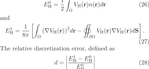
for DFT calculations. One way to assess the accuracy of the solution is by comparing the values of two expressions for the Hartree energy, namely
E0
H= 1 2
ˆ
Ω
VH(r)n(r)dr (26)
and
E1
H= 1 8π
ˆ
Ω
(∇VH(r))2dr−
‹
∂Ω
VH(r)∇VH(r)dS
.
(27) The relative discretization error, defined as
d=
E1
H−EH0
E0
H
(28)
can then serve as a measure of the inaccuracy of the solu-tion. Figure 3 shows how this error is unacceptably large when a second-order solver is used. The problem can be addressed by employing high-order defect correction, where higher-order finite differences are used to itera-tively correct the solution obtained with a second-order solver59. In this way the discretization error can be
sys-tematically reduced (Figure 3) with moderate computa-tional cost. No changes to the second-order solver are necessary. The computational cost of the multigrid ap-proach scales linearly with the volume of the simulation cell, albeit with a large prefactor.
10-6
10-5
10-4
10-3
10-2
10-1
2 4 6 8 10 12
Relative discretization error,
d
[image:8.595.54.298.466.580.2]FD order
Figure 3. Relative discretization error Eq. (28) in the Hartree energy vs. the order of the finite differences used in the de-fect correction of the second-order solution, on the example of aspartate. An order of 2 corresponds to the uncorrected solution. Smeared ions were used.
The multigrid method does not rely on any particular form of the Dirichlet boundary conditions specified on ∂Ω, however, to obtain a potential consistent with the OBCs used for the remaining energy terms, these should be
VH(r) =
ˆ
Ω n(r′)
|r−r′|dr
′ forr
∈∂Ω. (29)
Although the evaluation of the boundary conditions is straightforward, it is computationally costly, scaling un-favourably as O(L2V), which, for localised charge, im-plies O(L2N). To ameliorate this problem, a suitable coarse-grained approximation can be used instead of n(r′). Combined with evaluating Eq. (29) only for a sub-set of points in∂Ω and using interpolation in between, this leads to a reduction of the computational effort by 3-4 orders of magnitude, which brings it into the realm of feasibility.
The smeared-ion formalism60, where the total energy is
rewritten by adding and subsequently subtracting Gaus-sian charge distributions centred on the cores, can be used in conjunction with the multigrid approach. In this case, the Poisson equation, Eq. (6), is solved for the elec-trostatic potential generated by thetotal charge density
(due to electrons and smeared ions). As the cores neu-tralize a significant fraction of the electronic charge, the magnitude of the relevant quantities (charge density, po-tential) is smaller. Assuming the relative error incurred by the multigrid remains the same, this has the advan-tage of reducing the absolute error. The use of smeared ions, however, introduces approximations of its own. For a more detailed discussion of smeared ions the reader is referred to Ref.60. We shall evaluate the approach with
VI. CONVERGENCE PROPERTIES
A. Small Molecular Systems
We test these methods first on small-scale, simple sys-tems to demonstrate their equivalence in the limit that all relevant parameters are accurately converged. For this, we select a test set of small ions molecules: a phosphate ion (PO 3−
4 ), pyridinium (C5NH6)1+, the amino-acid salt aspartate with a charge of −1e, and the amino acid ly-sine with a charge of +1e, the neutral molecules water (H2O) and potassium chloride (KCl). In this set, we have thus included two cations, two anions and neutral molecules with a relatively low and a very high dipole moment, respectively. Clearly, these small molecules are unchallenging calculations for linear-scaling DFT, of a size below the onset of any linear-scaling behaviour, but they serve to illustrate the main convergence issues in a controllable way, since it is here possible to make the sim-ulation cell very much larger than the molecule, within feasible computational memory requirements. Illustra-tions are shown in Figure 4 of this test set.
Each molecule was simulated in a cubic simulation cell initially of size 32.5a0, with a grid spacing of 0.5a0 (equiv-alent to an energy cutoff of around 827eV), and with all NGWF radii set to 7.0a0. The density kernel was not truncated (all elements allowed to be nonzero) as the systems are too small for meaningful truncation. Norm-conserving pseudopotentials are employed for all the ions included here, and exchange-correlation is described by the PBE functional. We choose, throughout this work, to examine the convergence of the total energy, because although in practice one is most often interested in a quantity derived from it, such as formation or binding energies, the finite size errors made in total energies due to monopole or higher charges cannot be expected to can-cel between (for example) reactant and product states, so convergence of the total energy must be obtained individ-ually for each system.
B. Convergence
First, we examine the option of extrapolation to infi-nite size from calculations performed under PBCs. The black squares in Figure 5 show the uncorrected total en-ergy of each of the six molecular species, calculated under PBCs. According to Makov and Payne23, the total
en-ergy as a function of box size can be expected to behave approximately as
E=E0− q2α
2L −
2πqQ
3L3 +O(L
−5) (30)
in a cubic simulation cell of side L, where q is the to-tal charge, Q is the quadrupole moment, and α is the Madelung constant, where for cubic cells α ≃ 2.837. They suggest an approximate correction scheme based on
removing the leading orderL-dependent term. However, there are two options for going about this in practice.
Direct calculation of quadrupole moment Qfrom the density is problematic and a more reliable approach is to set the monopole chargeqaccording to the known charge and then fit E0 and Q to data using a least-squares fit to data at multiple values ofL. Alternatively, one could take into account that for a cell containing a molecule which is to some extent extended and may be somewhat polarisable, the mean dielectric constant is not equal to precisely unity. One could therefore also allow the co-efficient of the 1/L term to vary freely, and allow an O(L−5) coefficient as well. Examining Figure 5 we see that the finite size error for those species with a monopole charge follows E(L) = E0 +O(L−1) fairly well as ex-pected. The species with only a dipole moment (not a monopole) display a much weaker effect, which behaves asE(L) =E0+O(L−3). However, as the charge distri-bution varies withL, and so the coefficientQin Eq. (30) depends weakly onL, the fit to the Makov-Payne form is not exact. Nevertheless, in the smallcharged molecules
used here, the fitted Makov-Payne correction achieves a fairly well-defined correction to the total energy, aligning each individual energy to the extrapolated infinite-cell-size limit even for smaller cells, producing a good fit. However, the extra freedom allowed by varying q or in-troducingO(L−5)terms are seen to produce a less useful extrapolation, by fitting to noise. This can only be seen for sure by comparing to the known answer obtained un-der one of the correction schemes as seen below.
The effect of self-consistency in these small systems is not very strong: that is to say, the rearrangement of the charge due to the influence of the potential from neigh-bouring images of the cell is not very great. Henceforth, for Makov-Payne results, we will show thecorrected
re-sultEPBC(L)−EMP(L) +E0, whereEMP(L)is the ap-propriate Makov-Payne choice, as this result falls on a comparable scale to the results for the other schemes, enabling visual comparison.
Within the cutoff Coulomb approach, we can individ-ually vary the size of the original cell, the size of the padded cell, and the cutoff radius of the interaction. We note that the results obtained are converged to less than 1µeV/atom once the extent of the density of the molecule is less than that of the original cell. Since the interac-tion is constructed in reciprocal space but has a sharp cutoff in real space atRc, care must be taken to include sufficient padding that the cutoff falls within a vacuum region, and the region of ‘ringing’ induced by the cutoff is at least 5-10a0 from any significant values of nonzero density. Once this is achieved, residual variation of the result withRc is well below 1µeV/atom.
For the MIC approach, we obtain near-identical re-sults for our implementation of the Martyna-Tuckerman approach as compared to our implementation of the ap-proach of Genovese et. al. We thus only show the MT
Gen-Figure 4. (Color online) Small molecules for initial tests, covering anions and cations and species with dipole moments. From left to right: phosphate, pyridinium, aspartate, lysine, potassium chloride and water.
-1932.00 -1928.00 -1924.00 -1920.00 -1916.00
E
(eV)
-1916.40 -1916.38 -1916.36 -1916.34 -1916.32
20 30 40 50 60 70 80 90 100
E
(eV)
Cell side, L (a.u.)
-418.3500 -418.3400 -418.3300 -418.3200 -418.3100 -418.3000 -418.2900
E
(eV)
-418.3020 -418.3019 -418.3018 -418.3017 -418.3016 -418.3015 -418.3014
20 30 40 50 60 70 80 90 100
E
(eV)
Cell side, L (a.u.)
Figure 5. Convergence of total energy with simulation cell size for a monopolar system (PO3−
4 , left) and a dipolar system
(KCl, right), showing the uncorrected results in the upper panels, and different forms of Makov-Payne correction in the lower
panels: a) red squares: E(L) =E0+q2α/2L+B/L3; b) green triangles: E(L) =E0+A/L+B/L3+C/L5; c) blue circles:
E(L) =E0+B/L3; d) orange diamonds: E(L) =E0+B/L3+C/L5.
ovese et. al. approach is technically more sophisticated
and requires less computational effort overall due to the lower padding requirements. Martyna and Tuckerman note that to obtain accurate reciprocal-space representa-tion of the MIC Coulomb potential, a smaller grid spac-ing is sometimes required compared to the requirements of a comparable PBC calculation. Alternatively, one can represent just the density and potential on a finer grid. Taking the latter approach, we compared grid spacings 2.0×,2.5×and3.0×the underlying psinc grid for
repre-sentation of the density and potential. While the results do show minor variations (from 20 to 100µeV/atom de-pending on the system), this variation is present to the same extent also in PBC calculations so should not be at-tributed to the MT approach itself — rather it is thought to result from changing the grid in discrete evaluation of the XC energy integral. We thus employ the standard 2.0×fine grid spacing throughout the rest of this work.
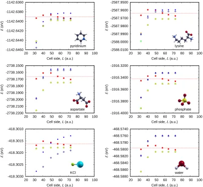
We show in Figure 6 the total energy of the test sys-tems evaluated all the above methods. The CC results use the spherical cutoff of Eq. (11). The results for the CC and MIC methods converge rapidly with system size to effectively the same value. In very small simulation cells, below 42a0, the extent of the ‘FFT box’ — and thus the total extent of the charge distribution — is the same as that of the simulation cell. In such cases, the sim-ulation cell contains very small contributions to the total electron density that wrap through the periodic bound-aries. Therefore, even the correction schemes do not fully account for the absense of periodic interactions, and a quite strong dependence on L at very small L is seen. However, as soon as the simulation cell is large enough
that the density is contained fully within one cell, the re-sult is beyond that point entirely converged with system size and independent ofL.
However, the OBC calculations evidently produce re-sults of a somewhat lower accuracy. For these re-sults, several distinct sources of inaccuracy can be dis-tinguished. First and foremost, the calculation of the local pseudopotential under OBCs is performed numer-ically and the associated error increases with the size of the simulation cell. The reasons behind this are ex-plained in detail in Appendix B. For the systems and box sizes encountered here, the magnitude of this error is20−200µeV/atom, thus it is only apparent in the plots for KCl, where the magnification is the highest. Second, the use of a multigrid approach to solve Eq. (6) introduces a discretization error. The magnitude of this error, how-ever, can be easily made negligible by employing high-order defect correction, and introducing smeared ions, as explained earlier in section V, cf. Fig. 3. Third, there are approximations involved in the generation of boundary conditions Eq. (29) for the solution of Eq (6). In our im-plementation we coarse-grain charge densities (electronic when smeared ions are not used, or total when using smeared ions) represented on a grid by replacing cubic blocks ofp×p×pgridpoints with a single point charge located at the centre of charge of the block (thus, in gen-eral, not at a gridpoint). This is only done when evaluat-ing the integral in Eq (29). Withp= 5(used throughout this work) the the prefactor for the calculation of the boundary conditions is reduced125-fold, whereas the as-sociated error in the energy was less than 75µeV/atom in the worst case (PO 3−
[image:10.595.82.543.139.281.2]di--1142.6460 -1142.6440 -1142.6420 -1142.6400 -1142.6380 -1142.6360
20 30 40 50 60 70 80 90 100
E
(eV)
Cell side, L (a.u.) pyridinium
-2588.0100 -2588.0000 -2587.9900 -2587.9800 -2587.9700 -2587.9600 -2587.9500
20 30 40 50 60 70 80 90 100
E
(eV)
Cell side, L (a.u.) lysine
-2738.2200 -2738.2100 -2738.2000 -2738.1900 -2738.1800 -2738.1700 -2738.1600 -2738.1500
20 30 40 50 60 70 80 90 100
E
(eV)
Cell side, L (a.u.) aspartate
-1916.4000 -1916.3800 -1916.3600 -1916.3400 -1916.3200
20 30 40 50 60 70 80 90 100
E
(eV)
Cell side, L (a.u.) phosphate
-418.3030 -418.3025 -418.3020 -418.3015 -418.3010
20 30 40 50 60 70 80 90 100
E
(eV)
Cell side, L (a.u.) KCl
-468.5880 -468.5860 -468.5840 -468.5820 -468.5800 -468.5780 -468.5760 -468.5740
20 30 40 50 60 70 80 90 100
E
(eV)
Cell side, L (a.u.) water
Figure 6. Convergence of total energy with simulation cell size for test molecules, using: Cutoff Coulomb (green circles), Martyna-Tuckerman (orange triangles), OBCs (blue diamonds, filled when smeared ions were used), and MP-corrected PBCs (red squares). CC and MT results rapidly approach the same converged answer once the size of the cell is greater than the extent of the density. This converged result agrees well with the trend of the MP-corrected lines. The OBC results are offset by a constant due to the approximations involved in the smeared-ion representation and by an error whose magnitude increases with the box size (particularly evident for KCl) as a consequence of the numerical evaluation of the real-space pseudopotential (see Appendix B).
minished quickly with increasing box sizes. For neutral systems, even with high dipole moments, this error was less than6µeV/atom, again quickly diminishing with the box size.
Finally, the introduction of smeared ions60 also affects
the obtained energies, as evidenced by the near-constant shifts between the results with and without smeared ions, observed in the plots. The error incurred by using smeared ions is due to the fact that certain terms in the formalism (e.g. the self-interaction of every smeared ion) are calculated analytically, whereas other terms (e.g. the local pseudopotential energy) are calculated by integrat-ing the relevant quantities on a grid. Thus, the terms that are meant to cancel only do so in the limit of an infinitely fine grid. For the systems discussed here, the residual error is100−300µeV/atom, outweighing the
re-duction in the other sources of error that smeared ions bring about – it is apparent from the plots that the cal-culations would be more accurate without smeared ions. Smeared ions find use in the context of implicit solvent calculations61, as they allow the dielectric continuum to
polarise in response not only to the electronic density, but also to the density of the smeared cores. For calcu-lations in vacuum involving the systems of interest here, their introduction negatively impacted accuracy.
[image:11.595.110.514.56.428.2]tends to worsen results. Finally, when using OBCs, the energy is actually expected to very slowly diverge with the size of the simulation cell, due to the inaccuracies involved in the evaluation of the local pseudopotential. This effect, compounded by the near-constant shift due to the use of smeared ions means that OBC results should only be compared against other OBC results rather than results from PBC calculations.
VII. LARGE SYSTEMS AND
COMPUTATIONAL OVERHEAD
To validate and compare these methods in a more real-istic setting, it is necessary to examine their performance in larger-scale systems more typical of the real applica-tions of linear-scaling DFT. These will often behave very differently from very small systems, because it is usually impossible to perform the calculations in a simulation cell where the dimensions of the cell greatly exceed that of the molecule or nanostructure. Furthermore, the scaling of the computational effort with system size may be very different as the balance of time spent in different parts of the calculation changes with the number of atoms.
To demonstrate the accuracy of the methods, and the computational overhead and the scaling of each of these approaches, we have simulated two fairly large sys-tems, each comprising around 1250 atoms, which for these systems is well above the threshold at which linear-scaling methods offer a clear advantage in terms of re-duced computational effort over comparable traditional DFT approaches. These systems are: a fragment of the L99A/M102Q mutant of the T4 Lysozyme protein61,62,
and a nanocrystal of gallium arsenide in the wurtzite structure, with hydrogen termination63. Figure 7
illus-trates these systems.
The protein fragment has a high net charge of+7eas a result of the protonation state of its residues at nor-mal pH, and hence displays a strong finite size effect on the total energy if periodic boundary conditions are em-ployed. This makes it difficult to calculate meaningful binding energies of ligands to its polar binding site. The distribution of the net charge is largely determined by the functional groups included and to a great extent it can be viewed as localised on these groups, so it is not expected to depend strongly on the system size: to a reasonable approximation we can treat the density of this system as fixed when we vary the size of the simulation cell.
The GaAs nanorod, on the other hand, has no net charge, but the underyling wurtzite structure, with no inversion symmetry, means that when truncated at each end of the rod along the c-axis, Ga and As faces are exposed on opposite ends of the rod. No matter how the surface is terminated (in the case studied here, all dangling bonds are saturated with hydrogen), there will be some form of charge transfer between the ends and a dipole moment along thec-axis will result. If such a rod is simulated in a box of size comparable to the rod itself
Figure 7. Illustration of test set of large systems (a)
1234-atom fragment of the L99A/M102Q mutant of the T4 Lysozyme protein (b) Wurtzite-structure GaAs Nanorod of 1284 atoms, with hydrogen atoms terminating dangling bonds.
under PBCs, then the rod is effectively surrounded by an inifinite array of replicas, producing a very different elec-tric field from that of an isolated rod. Indeed, unless the box is very large along all axes, the Ga-terminated end of the rod will be in closer proximity to the As-terminated ends of rods in adjacent cells than to the As-terminated end on the on the same rod (and vice versa), and the rod is strongly polarisable. This is clearly a very dif-ferent situation from the ideal situation many correction methods assume, of a strongly localised fixed charge dis-tribution in a box considerably larger than the charge distribution itself. Because the magnitude of the dipole moment depends sensitively on the balance of charge dis-tribution and the density of states at the polar surfaces of the rod, its value can be affected by the field created by the charge distribution of periodic images of the rod, bringing self-consistent effects into play.
To perform these large simulations, we use in both cases a grid spacing of 0.5a0, equivalent to a plane-wave cutoff of around 827eV, and standard well-tested norm-conserving pseudopotentials for each species. For the protein system, four NGWFs of radius 7.0a0 were placed on each C, N, O and S atom, and one on each H atom. For the nanorod, larger NGWFs were required to achieve good convergence, so Rφ = 10a0 was used, with four NGWFs on Ga and As and one on H.
The total energy of the the protein fragment as a func-tion of supercell side length is shown in Figure 8. We use a series of cells up to L = 400a0 in size, so as to be able to accurately extrapolate to L → ∞. We see
de--144400.0 -144390.0 -144380.0 -144370.0 -144360.0 -144350.0
E
(eV)
-144368.0 -144367.8 -144367.6 -144367.4 -144367.2
100.0 200.0 300.0 400.0 500.0
E
(eV)
[image:13.595.66.289.54.200.2]Cell side, L (a.u.)
Figure 8. Convergence of total energy with cell size for
T4 lysozyme fragment, showing results for Cutoff Coulomb (green circles), Minimum Image Convention (orange trian-gles), Open Boundary Conditions (blue diamonds, filled when smeared ions were used) and Periodic Boundary Conditions (red squares) corrected using the Makov-Payne form (a) fitted
by least-squares fitting toE0 andB.
tails: firstly, there remains considerable residual varia-tion in the Makov-Payne corrected results, which do not converge to better than 0.05eV untilL = 200a0. When they do so, they agree well with the MP extrapolation. The OBC result suffers from considerable residual error, mostly due to the approximations involved in the evalu-ation of the local pseudopotential, which for the smaller box sizes cancels out, to a degree, with the error due to the approximations in the construction of the bound-ary conditions, but for larger boxes causes the energy to very slowly diverge. The almost constant shift in en-ergy incurred by the use of smeared ions is approximately 400µeV/atom. The CC and MT results agree very well with each other, to around the 1meV level. We conclude that for monopolar systems with an approximately fixed charge distribution, the CC and MT methods are both reliable as long as the cell is made large enough for the conditions of each method to hold.
The total energy of the the nanorod as a function of supercell side length is shown in Figure 9. Here the de-fault supercell is not chosen to be cubic as this would be particularly inefficient for such a high-aspect ratio nanos-tructure. We start with Lx = 240a0, Ly, Lz = 65a0 as the smallest cell able to completely enclose the rod with around10a0 padding in all directions, and then Ly and
Lz are scaled commensurately with Lx. We see that in this case, with a highly polarisable rod, the same Makov-Payne fit that successfully described the dipolar systems in Section VI now fails significantly for all the cells stud-ied here and returns an E0 which does not match the L→ ∞limit, nor does it match the CC or MIC results. The latter are well-converged with respect toLx, and are in good agreement with each other. However, again the OBC results are strongly size-dependent, as a result of the approximations made in order to obtain feasible com-putational effort at this large scale. The validity of the
-200614.5 -200614.0 -200613.5 -200613.0 -200612.5
200 300 400 500 600 700 800 900 1000
E
(eV)
Cell side, Lx (a.u.)
[image:13.595.340.545.55.175.2]GaAs nanorod
Figure 9. Convergence of total energy with cell size for GaAs Nanorod, showing results for Cutoff Coulomb (green circles), Minimum Image Convention (orange triangles), Open Bound-ary Conditions (blue diamonds, filled when smeared ions were used) and Periodic Boundary Conditions (red squares) cor-rected using the Makov-Payne form (c) fitted by least-squares
fitting toE0 andB. CC results are independent of cell size
for allLxgreater than the rod length. The MIC approach
re-quiresLx>2×Lrod, so results are only shown forLx≥480a0.
convergence of the approximate methods starts to break down beyondLx∼300a0, resulting in significant error.
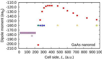
By examining the behaviour of the dipole moment of the rod along its length, calculated asdx=
´
Ωx n(r) dr, we see immediately why this is the case: the dipole mo-ment varies strongly with cell size because of the induced polarisation caused by the periodic images, as seen in Figure 10. The periodic images of the nanorods are all aligned, so if the rods are very close end-to-end they will tend to increase the dipole moment. However, if they are closer side-to-side the dipole field of the periodic image (in the opposite direction to the polarisation, as viewed outside the rod to its side) will tend to depolarise the rod and the dipole moment will decrease. Therefore there is a strong dependence ofdxon bothLx andLy, Lz. Both of these are spurious effects when one wishes to simulate an isolated rod. We see that all three approaches, CC, MIC, and OBC, all correct these influences and obtain the ‘correct’ isolated result fordxeven for small system sizes.
We therefore conclude that in such cases of large, po-larisable systems with a strong dipole moment, there is no choice but to use an approach including the truncation of periodic images: in analogy to the study of polar thin films26, a correction schememust be employed if reliable
-210.0 -200.0 -190.0 -180.0 -170.0 -160.0 -150.0 -140.0 -130.0 -120.0 -110.0
0 100 200 300 400 500 600 700 800 900 1000
Dipole moment (ea
0
)
Cell side, Lx (a.u.)
[image:14.595.76.280.56.175.2]GaAs nanorod
Figure 10. Dipole momentdx (see text) as a function of cell
size Lx for a GaAs nanorod. Here the inset illustration is
shown approximately to-scale with theL-axis. The exact form
ofdx(L)would depend on aspect ratio, and would be difficult
to accurately extrapolate to L → ∞. The cutoff Coulomb
and MIC approaches obtain converged results for all cell sizes large enough for their methods to hold, while the periodic results converge only very slowly to this isolated value.
simulation cells the energy inevitably diverges. Although this divergence is slow (compared to the total energy of the system), in the absence of a monopole charge and the associated O(L−1) term it makes the OBC results unacceptably inaccurate for energies. Figure 10 shows nevertheless that for other physical properties, such as the dipole moment, it may be reliable.
VIII. CONCLUSIONS
We have described and applied three different meth-ods, each with a rather different theoretical basis, to the study of calculations on charged and dipolar systems using linear-scaling density functional theory under pe-riodic boundary conditions. We have shown that with each of these methods it is possible, while staying within a nominally periodic formalism, to achieve the desired limit of equivalence of any calculated properties to those of a single isolated system.
In small systems, post-hoc correction schemes are
ca-pable of extrapolating to the isolated limit on the basis of several calculations performed under PBCs, but only if simulation cells are used which are very large com-pared to the system being studied. The first-order term of the Makov-Payne correction, on its own, is inadequate for accurate results, but by fitting the coefficient of the O(L−3)term, one can acheive an accurate result for a cu-bic cell as long as there is not a dipole moment present of comparable physical size to the cell itself. This is clearly a highly computational expensive approach due to the need to simulate several large cells to achieve an accu-rate fit, and is not really practical for production calcu-lations. Fitting further coefficients of the Makov-Payne expansion tends to reduce the accuracy by over-fitting to numerical noise.
However, we have also seen that the larger systems encountered in large linear-scaling DFT calculations can behave very differently from the small molecules in the test set. In particular, there is scope in large systems for considerable long-range charge redistributionin response to the effect of periodic images, so reliable extrapolation
from simulations using a small unit cell are then impos-sible. In such situations, one has no choice but to use a method that explicitly negates the effect of periodic images.
Approaches which redefine the Coulomb potential to avoid periodic interactions, either by using the Mini-mum Image Convention (whether in the form proposed by Martyna and Tuckerman, or in the rather different form by Genoveseet al.) or the cutoff Coulomb method,
have been seen to rapidly converge to the isolated result as soon as the conditions required as outlined above are met. In the case of the MT formulation, this is that the size of the simulation cell be at least twice the extent of the electron density in a given direction, while in the Genovese form, this requirement is relaxed due to the method being performed on what is effectively a padded real-space grid.
The cutoff Coulomb approach is seen to produce ac-curately converged results for a single-shot calculation, regardless of the size of the simulation cell (as long as it is bigger than the extent of the nonzero density). The only requirement is that the original cell must, for the purposes of Fourier transforms, be embedded in a padded cell of sufficient size. This generally entails quite a large temporary memory requirement, and in small systems the performance of FFTs can become the limiting factor on the speed of the whole calculation. However, in large systems, where the Hartree calculation is generally not a significant part of the total computational effort, this is no longer an issue.
We noted also that two of the methods considered here can benefit from similar speedups by suitable treatment of Fourier transforms padded with zeroes. In both the cutoff Coulomb approach and the MIC approach, there is a need to perform a FFT of the charge density to re-ciprocal space under conditions where the value on most of the real-space grid is known to be zero. In such cases, it has been shown that algorithms can be designed which not only significantly reduce the computational expense of such a transform but also reduce the memory usage by not explicitly storing the zeros. The MIC implemen-tation of Genoveseet al. employs such an approach, but
the Martyna-Tuckerman and cutoff Coulomb approaches could in principle also do so. This would render them all very similar in terms of computational cost, only marginally above that of the original, uncorrected ap-proach.
ACKNOWLEDGMENTS
N.D.M.H and J.D. acknowledge the support of the En-gineering and Physical Sciences Research Council (EP-SRC Grant Nos. EP/F010974/1, EP/G05567X/1 and EP/G055882/1) for postdoctoral funding through the HPC Software Development call 2008/2009. P.D.H. and C.-K.S. acknowledge support from the Royal Society in the form of University Research Fellowships. The au-thors are grateful for the computing resources provided by Imperial College’s High Performance Computing ser-vice (CX2), and by Southampton’s iSolutions (Iridis3) which have enabled all the simulations presented here. We would like to thank Stephen Fox for the structure of the T4 lysozyme and Philip Avraam for the structure of the GaAs nanorod.
APPENDIX A: FOURIER COEFFICIENTS OF THE CYLINDRICALLY-CUTOFF
INTERACTION
The integral for the Fourier components˜vCC(G)of the Coulomb interaction cut off over a cylinder of length2L and radiusRcan be written
˜
vCC(G) =
ˆ
cyl
eiG.r
r dr
=
ˆ R
0
ˆ L
−L
ˆ 2π
0
ρ ei(Gρρsinφ+Gxx)
p
ρ2+x2 dφdxdρ .
Here we have taken the cylinder to be aligned along x, and takenGρto lie in thexy-plane, without loss of gener-ality. To ensure that the resulting expression is finite and well-behaved for all non-negative values ofG, we identify
four regions which must be treated separately:
Gρ>0, Gx>0;
Gρ= 0, Gx>0;
Gρ>0, Gx= 0;
Gρ= 0, Gx= 0.
The latter three cases all allow significant simplification of the integral and will be examined first.
TheGρ= 0, Gx= 0terms are the only ones where the integral can be performed fully analytically:
˜
vCC(G) =
ˆ R
0
ˆ L
−L
ˆ 2π
0
ρ
p
ρ2+x2dφdxdρ
= 4π
ˆ R ρ=0 ˆ L x=0 ρ p
ρ2+x2dxdρ
= 4π
ˆ L
0
p
R2+x2−xdx
= 2πhL(pR2+L2−L) +R2ln
"
L+√R2+L2 R
# i
The Gρ = 0, Gx > 0 terms can be rendered into a well-behaved integral overx:
˜
vCC(G) =
ˆ R
0
ˆ L
−L
ˆ 2π
0
ρ eiGxx
p
ρ2+x2dφdxdρ
= 4π
ˆ R
0
ˆ L
0
ρcosGxx
p
ρ2+x2dxdρ
= 4π
ˆ L
0
p
R2+x2−xcosG xxdx
which can be evaluated numerically with no significant difficulties
Similarly, theGρ>0, Gx= 0terms can be made into a well-behaved integral overρ:
˜
vCC(G) =
ˆ R
0
ˆ L
−L
ˆ 2π
0
ρ eiGρρsinφ
p
ρ2+x2 dφdxdρ
= 2
ˆ R
0
ˆ L
0
ˆ 2π
0
ρcos[Gρρsinφ]
p
ρ2+x2 dφdxdρ
= 4π
ˆ R 0 ˆ L 0 ρ p
ρ2+x2J0(Gρρ) dxdρ
= 2π
ˆ R
0 ln
"
L+p
ρ2+L2
−L+pρ2+L2
#
ρ J0(Gρρ) dρ.
which also remains well-behaved over its range.
the integrals become tractable, then the resulting answer can be convolved with a top-hat function to retrieve the desired limits on the integral. The top hat function is defined in terms of the Heaviside step function:
T(r) = Θ(x+L)−Θ(x−L).
The transform of the Coulomb interaction for the infinite cylinder would give
˜
vIC(G) =
ˆ R
0
ˆ ∞
−∞
ˆ 2π
0
ρ eiGρρsinφ+iGxx
p
ρ2+x2 dφdxdρ ,
so we can write the transform of the finite cylinder as
˜
vCC(G) =
ˆ R
0
ˆ ∞
−∞
ˆ 2π
0
T(r)vIC(r)ei(Gρρsinφ+Gxx)dφdxρdρ .
By the convolution theorem we can write the transform of the product of two functions in real space as the con-volution of these two functions in reciprocal space. Using
Hfor our primed set of reciprocal space coordinates we
get:
˜
vCC(G) = 1 (2π)3
ˆ
˜
vIC(H) ˜T(G−H) d3H.
All three integrals forv˜IC(H)can be done analytically:
˜
vIC(H) =
ˆ R
0
ˆ ∞
−∞
ˆ 2π
0
ρ
p
ρ2+x2cos(Hxx) cos(Hρρsinφ) dφdxdρ
= 2
ˆ R
0
ˆ 2π
0
ρ K0(Hxρ) cos(Hρρsinφ) dφdρ
= 4π
ˆ R
0
ρ K0(Hxρ)J0(Hρρ) dρ
= 4π
1 +HρR K0(HxR)J1(HρR)−HxR K1(HxR)J0(HρR)
H2 ρ+Hx2
This expression is in fact very simple to evaluate as it contains no Bessel functions of higher order than 1. These can be rapidly evaluated using accurate polyno-mial approximations over the domain required for the integrals.
For the step function, the transform is well known
˜
T(G) = ˆ L
−L
exp[iGxx]dx δ(Gρ)
= 2 sin(GxL)
Gx
δ(Gρ).
Combining the two gives us
˜
vCC(G) = 1 (2π)3
ˆ 2 sin[(G
x−Hx)L]
Gx−Hx
δ(Gρ−Hρ)˜vIC(H) d3H.
After performing theHρ integral to leave onlyHρ =Gρ, we obtain
˜
vCC(G) = 4
ˆ ∞
−∞
sin[(Gx−Hx)L] (Gx−Hx)
×
1 +G
ρR K0(HxR)J1(GρR)−HxR K1(HxR)J0(GρR)
G2 ρ+Hx2
dHx
= 4π
(G2 x+G2ρ)
×
1−e−GρL(Gx Gρ
sinGxL−cosGxL)
+4
ˆ ∞
−∞
sin[(Gx−Hx)L][GρR K0(HxR)J1(GρR)−HxR K1(HxR)J0(GρR)] (Gx−Hx)(G2ρ+Hx2)
dHx