A new approach to the treatment of Separatrix Chaos and its applications

University of Warwick institutional repository: http://go.warwick.ac.uk/wrap

This paper is made available online in accordance with

publisher policies. Please scroll down to view the document

itself. Please refer to the repository record for this item and our

policy information available from the repository home page for

further information.

To see the final version of this paper please visit the publisher’s website.

Access to the published version may require a subscription.

Author(s):

S.M. Soskin, R. Mannella, O.M. Yevtushenko, I.A.

Khovanov, P.V.E. McClintock

Chapter details: A New Approach to the Treatment of Separatrix

Chaos and Its Applications, In: Hamitonian Chaos Beyond the KAM

Theory, Dedicated to George M. Zaslavsky (1935—2008)

Year of publication: 2010

Link to published article:

http://www.springer.com/new+&+forthcoming+titles+(default)/book/978

-3-642-12717-5

A New Approach To The Treatment Of

Separatrix Chaos And Its Applications

S.M. Soskin, R. Mannella, O.M. Yevtushenko, I.A. Khovanov, P.V.E. McClintock

AbstractWe consider time-periodically perturbed 1D Hamiltonian systems

pos-sessing one or more separatrices. If the perturbation is weak, then the separatrix chaos is most developed when the perturbation frequency lies in the logarithmically small or moderate ranges: this corresponds to the involvement of resonance dynam-ics into the separatrix chaos. We develop a method matching the discrete chaotic dynamics of the separatrix map and the continuous regular dynamics of the reso-nance Hamiltonian. The method has allowed us to solve the long-standing problem of an accurate description of the maximum of the separatrix chaotic layer width as a function of the perturbation frequency. It has also allowed us to predict and de-scribe new phenomena including, in particular: (i) a drastic facilitation of the onset of global chaos between neighbouring separatrices, and (ii) a huge increase in the size of the low-dimensional stochastic web.

S.M. Soskin

Institute of Semiconductor Physics, 03028 Kiev, Ukraine, e-mail: [email protected]

R. Mannella

Dipartimento di Fisica, Universit`a di Pisa, 56127 Pisa, Italy, e-mail: [email protected]

O.M. Yevtushenko

Physics Department, Ludwig-Maximilians-Universit¨at M¨unchen, D-80333 M¨unchen, Germany, e-mail: [email protected]

I.A. Khovanov

School of Engineering, University of Warwick, Coventry CV4 7AL, UK, e-mail: [email protected]

P.V.E. McClintock

Physics Department, Lancaster University, Lancaster LA1 4YB, UK, e-mail: [email protected]

Contents

1 Introduction. . . .

1.1 Heuristic results. . . .

1.2 Mathematical and accurate physical results . . . .

1.3 Numerical evidence for high peaks in∆E(ωf)and

their rough estimation . . . .

1.4 Accurate description of the peaks and of the related

phenomena. . . .

2 Basic ideas of the approach. . . .

3 Single-Separatrix Chaotic Layer. . . .

3.1 Rough estimates. Classification of systems. . . .

3.2 Asymptotic theory for systems of type I.. . . .

3.3 Asymptotic theory for systems of type II.. . . .

3.4 Estimate of the next-order corrections . . . .

3.5 Discussion. . . . 4 Double-separatrix chaos . . . . 4.1 Asymptotic Theory For The Minima Of The Spikes . . . . . 4.2 Theory of the Spikes’ Wings . . . . 4.3 Generalizations and Applications . . . . 5 Enlargement of a low-dimensional stochastic web . . . . 5.1 Slow modulation of the wave angle . . . . 5.2 Application to semiconductor superlattices . . . . 5.3 Discussion . . . . 6 Conclusions . . . . 7 Appendix . . . . 7.1 Lower chaotic layer . . . . 7.2 Upper chaotic layer . . . .

References . . . .

1 Introduction

Separatrix chaos is the germ of Hamiltonian chaos [51]. Consider an integrable Hamiltonian system possessing a saddle, i.e. a hyperbolic point in the one-dimensional case, or a hyperbolic invariant torus, in higher-dimensional cases. The stable (in-coming) and unstable (outgoing) manifolds of the saddle are called separatrices [18]: they separate trajectories that have different phase space topologies. If a weak time-periodic perturbation is added, then the separatrix is destroyed; it is replaced by aseparatrix chaotic layer(SCL) [51, 18, 23, 29]. Even if the unperturbed system

1_{This version of the chapter represents just about 1/3 of the text in order to accord the copyright}

does not possess a separatrix, the resonant part of the perturbation generates a sepa-ratrix in the auxiliary resonance phase space while the non-resonant part of the per-turbation destroys this separatrix, replacing it with a chaotic layer [51, 18, 23, 10]. Thus separatrix chaos is of a fundamental importance for Hamiltonian chaos.

One of the most important characteristics of SCL is its width in energy (or ex-pressed in related quantities). It can be easily foundnumericallyby integration of the Hamiltonian equations with a set of initial conditions in the vicinity of the sep-aratrix: the space occupied by the chaotic trajectory in the Poincar´e section has a higher dimension than that for a regular trajectory, e.g. in the 3/2D case the regular trajectories lie on lines i.e. 1D objects while the chaotic trajectory lies within the SCL i.e. the object outer boundaries of which limit a 2D area.

On the other hand, it is important to be able to describe theoreticallyboth the outer boundaries of the SCL and its width. There is a long and rich history of the such studies. The results may be classified as follows.

1.1 Heuristic results

Consider a 1D Hamiltonian system perturbed by a weak time-periodic perturbation:

H=H0(p,q) +hV(p,q,t), (1)

V(p,q,t+2π/ωf) =V(p,q,t), h¿1,

whereH0(p,q)possesses a separatrix and, for the sake of notational compactness, all relevant parameters ofH0andV, except possibly forωf, are assumed to be∼1.

Physicists proposed a number of different heuristic criteria [53, 10, 23, 55, 51, 52] for the SCL width∆E in terms of energyE ≡H0(p,q)which gave qualitatively similar results:

∆E≡∆E(ωf)∼ωfδ, (2)

δ≡h|ε|,

|ε|∼<1 for ωf ∼<1, |ε|∝exp(−aωf)¿1 (a∼1) for ωf À1.

The quantityδ ≡h|ε|is called theseparatrix split[51] (see also Eq. (4) below): it determines the maximum distance between the perturbed incoming and outgoing separatrices [53, 10, 23, 55, 51, 52, 1, 18, 29].

It follows from (2) that the maximum of∆E should lie in the frequency range ωf ∼1 while the maximum itself should be∼h:

∆Emax≡max

ωf {∆E(ωf)} ∼h, ω

(max)

1.2 Mathematical and accurate physical results

Many papers studied the SCL by mathematical or accurate physical methods. For the rangeωf À1, many works studied the separatrix splitting (see the review

[18] and references therein) and the SCL width in terms of normal coordinates (see the review [29] and references therein). Though quantities studied in these works differ from those typically studied by physicists [53, 10, 23, 55, 51, 52], they im-plicitly confirm the main qualitative conclusion from the heuristic formula (2) in the high frequency range: provided thatωf À1 the SCL width is exponentially small.

There were also several works studying the SCL in the opposite (i.e. adiabatic) limit ωf →0: see e.g. [27, 14, 28, 42, 45] and references therein. In the context

of the SCL width, it is most important that∆E(ωf →0)∼h for most of the

sys-tems [27, 14, 28]. For a particular class of syssys-tems, namely for ac-driven spatially periodic systems (e.g. the ac-driven pendulum), the width of the SCL part above the separatrix diverges in the adiabatic limit [42, 45]: the divergence develops for ωf ¿1/ln(1/h).

Finally, there is a qualitative estimation of the SCL width for the rangeωf ∼1

within the Kolmogorov-Arnold-Moser (KAM) theory [29]. The quantitative esti-mate within the KAM theory is lacking, apparently being very difficult for this fre-quency range [17]. It follows from the results in [29] that the width in this range is of the order of the separatrix split, which itself is of the order ofh.

Thus it could seem to follow that, for all systems except ac-driven spatially peri-odic systems, the maximum in the SCL width is∼hand occurs in the rangeωf∼1,

very much in agreement with the heuristic result (3). Even for ac-driven spatially periodic systems, this conclusion could seem to apply to the width of the SCL part below the separatrix over the whole frequency range, and to the width of the SCL part above the separatrix forωf ∼>1/ln(1/h).

1.3 Numerical evidence for high peaks in

∆

E

(ω

)

and their rough

estimation

The above conclusion disagrees with several numerical studies carried out during the last decade (see e.g. [42, 45, 34, 25, 40, 24, 47, 35]) which have revealed the existence of sharp peaks in∆E(ωf)in the frequency range 1/ln(1/h)∼<ωf ∼<1 the

heights of which greatly exceedh(see also Figs. 2, 3, 5, 6 below). Thus, the peaks represent the generaldominant featureof the function∆E(ωf). They were related

1.4 Accurate description of the peaks and of the related

phenomena

Until recently, accurate analytic estimates for the peaks were lacking. It is explic-itly stated in [24] that the search for the mechanism through which resonances are involved in separatrix chaos, and for an accurate analytic description of the peaks in the SCL width as function of the perturbation frequency, are being among the most important and challenging tasks in the study of separatrix chaos. The first step towards accomplishing them was taken through the proposal [43, 44] of a new approach to the theoretical treatment of the separatrix chaos in the relevant fre-quency range. It was developed and applied to the onset of global chaos between two close separatrices. The application of the approach [43, 44] to the commoner single-separatrix case was also discussed. The approach has been further developed [38, 39], including an explicit theory for the single-separatrix case [39].

The present paper reviews the new approach [43, 44, 38, 39] and its applications to the single-separatrix [39] and double-separatrix [43, 44] cases. We also briefly review application to the enlargement of the low-dimensional stochastic web [46] and discuss other promising applications.

Though the form of our treatment differs from typical forms of mathematical the-orems in this subject (cf. [18, 29]), it yields theexactexpressions for the leading term in the relevant asymptotic expansions (the parameter of smallness isα≡1/ln(1/h)) and, in some case, even for the next-order term. Our theory is in excellent agreement with results obtained by numerical integration of the equations of motion.

Sec. 2 describes the basic ideas underlying the approach. Sec. 3 is devoted to the leading-order asymptotic description of the single-separatrix chaotic layers. Sec. 4 presents an asymptotic description of the onset of global chaos in between two close separatrices. Sec. 5 describes the increase in sizes of a stochastic web. Conclusions are drawn in Sec. 6. Sec. 7 presents the Appendix, which explicitly matches the separatrix map and the resonance Hamiltonian descriptions for the double-separatrix case.

2 Basic ideas of the approach

The new approach [43, 44, 38, 39] may be formulated briefly as a matching between the discrete chaotic dynamics of the separatrix map in the immediate vicinity of the separatrix and the continuous regular dynamics of the resonance Hamiltonian be-yond that region. The present section describes the general features of the approach in more detail.

approximation of motion near the separatrix in the asymptotic limit h→0, and an estimate of the error was also carried out in [31] (see also the review [29] and references therein).

The main ideas that allow one to introduce the SM [53, 10, 23, 55, 51, 52, 1, 29, 43, 44, 31] are as follows. For the sake of simplicity, let us consider a perturbation V that does not depend on the momentum:V ≡V(q,t). A system with energy close to the separatrix value spends most of its time in the vicinity of the saddle(s), where the velocity ˙qis exponentially small. DifferentiatingE≡H0(p,q)with respect to time and allowing for the equations of motion of the system (1), we can show that dE/dt ≡∂V/∂qq˙∝q. Thus, the perturbation can significantly change the energy˙ only when the velocity is not small i.e. during the relatively short intervals while the system is away from the saddle(s): these intervals correspond topulsesof velocity as a function of time (cf. Fig. 20 in the Appendix below). Consequently, it is pos-sible to approximate the continuous Hamiltonian dynamics by a discrete dynamics which maps the energyE, the perturbation angleϕ ≡ωft, and the velocity sign

σ≡sgn(q), from pulse to pulse.˙

The actual form of the SM may vary, depending on the system under study, but its features relevant in the present context are similar for all systems. For the sake of clarity, consider the explicit case when the separatrix ofH0(p,q)possesses a single saddle and two symmetric loops whileV =qcos(ωft). Then the SM reads [43] (cf.

Appendix):

Ei+1=Ei+σihεsin(ϕi), (4)

ϕi+1=ϕi+ωfπ(3−_2ω(Esgn(Ei+1−Es))

i+1) ,

σi+1=σisgn(Es−Ei+1), |σi|=1,

ε≡ε(ωf) =sgn µ

∂H0 ∂p

¯ ¯ ¯ ¯

t→−∞

¶Z _∞

−∞dt

∂H0 ∂p

¯ ¯ ¯ ¯ Es

sin(ωft),

Ei≡H0(p,q)|ti−∆, ϕi≡ωfti, σi≡sgn

Ã

∂H0 ∂p

¯ ¯ ¯ ¯ ti

!

,

whereEsis the separatrix energy,ω(E)is the frequency of oscillation with energy

E in the unperturbed case (i.e. forh=0),tiis the instant corresponding to thei-th

turning point in the trajectoryq(t)(cf. Fig. 20 in the Appendix below), and ∆ is an arbitrary value from the range of time intervals which greatly exceed the char-acteristic duration of the velocity pulse while being much smaller than the interval between the subsequent pulses [53, 10, 23, 55, 51, 52, 1, 29, 31]. Consider the two most general ideas of our approach.

1. If a trajectory of the SM includes a state withE=Es and an arbitraryϕ andσ,

then this trajectory is chaotic. Indeed, the angleϕof such a state is not correlated with the angle of the state at the previous step of the SM, due to the divergence ofω−1_(E→E

multiple of 2πby an arbitrary value. Hence the energy of the state at the previous step may deviate fromEsby an arbitrary value within the interval[−h|ε|,h|ε|].

The velocity signσis not correlated with that at the previous step either2_{. Given} that a regular trajectory of the SM cannot include a step where all three variables change random-like, we conclude that such a trajectory must be chaotic. Though the above arguments may appear to be obvious, they cannot be consid-ered a mathematically rigorous proof, so that the statement about the chaotic nature of the SM trajectory which includes any state withE=Esshould be

con-sidered as a conjecture supported by the above arguments and by numerical it-eration of the SM. Possibly, a mathematically rigorous proof should involve an analysis of the Lyapunov exponents for the SM (cf. [23]) but this appears to be a technically difficult problem. We emphasize however that a rigorous proof of the conjecture is not crucial for the validity of the main results of the present pa-per, namely for theleadingterms in the asymptotic expressions describing (i) the peaks of the SCL width as a function of the perturbation frequency in the single-separatrix case, and (ii) the related quantities for the double-single-separatrix case. It will become obvious from the next item that, to derive the leading term, it is suffi-cient to know that the chaotic trajectory does visit areas of the phase space where the energy deviates from the separatrix by values of the order of the separatrix splitδ≡h|ε|, which is a widely accepted fact [53, 10, 23, 55, 51, 52, 1, 18, 29].

2. It is well known [53, 10, 23, 55, 51, 52, 1, 18, 29, 34, 35, 43, 44], that, at the leading-order approximation, the frequency of eigenoscillation as function of the energy near the separatrix is proportional to the reciprocal of the logarithmic factor

ω(E) = bπω0 ln

³

∆H

|E−Es|

´, b=3−sgn(E−Es)

2 , (5)

|E−Es| ¿∆H≡Es−Est,

whereEst is the energy of the stable states.

Given that the argument of the logarithm is large in the relevant range of E, the function ω(E) is nearly constant for a substantial variation of the argu-ment. Therefore, as the SM maps the state(E0=Es,ϕ0,σ0)onto the state with E=E1≡Es+σ0hεsin(ϕ0), the value ofω(E)for the given sgn(σ0εsin(ϕ0))is nearly the same for most of the anglesϕ0(except in the vicinity of multiples of π),

ω(E)≈ωr(±), (6)

2_{Formally, sgn(E−E}

s)is not defined forE=Esbut, if to shiftEfromEsfor an infinitesemal

value, sgn(E−Es)acquires a value equal to either+1 or−1, depending on the sign of the shift.

Given thatσi+1is proportional to sgn(Es−Ei+1)while the latter is random-like (as it has been

ωr(±)≡ω(Es±h), sgn(σ0εsin(ϕ0)) =±1.

Moreover, if the deviation of the SM trajectory from the separatrix increases fur-ther,ω(E)remains close toωr(±)provided the deviation is not too large, namely

if ln(|E−Es|/h)¿ln(∆H/h). Ifωf ∼<ωr(±), then the evolution of the SM (4)

may be regular-like for a long time until the energy returns to the close vicinity of the separatrix, where the trajectory becomes chaotic. Such behavior is espe-cially pronounced if the perturbation frequency is close toωr(+) or ωr(−) or to

one of their multiples of relatively low order: the resonance between the pertur-bation and the eigenoscillation gives rise to an accumulation of energy changes for many steps of the SM, which results in a deviation ofEfromEsthat greatly

exceeds the separatrix split h|ε|. Consider a state at the boundary of the SCL. The deviation of energy of such a state fromEs depends on its position at the

boundary. In turn, the maximum deviation is a function ofωf. The latter

func-tion possesses the absolute maximum atωf close toωr(+)orωr(−)typically3, for

the upper or lower boundary of the SCL respectively. This corresponds to the absorption of the, respectively upper and lower, 1st-order nonlinear resonance by the SCL.

The second of these intuitive ideas has been explicitly confirmed [43] (see Ap-pendix): in the relevant range of energies, the separatrix map has been shown to reduce to two differential equations which are identical to the equations of motion of the auxiliary resonance Hamiltonian describing the resonance dynamics in terms of the conventional canonically conjugate slow variables, actionI and slow angle

˜

ψ ≡nψ−ωft whereψ is the angle variable [10, 23, 55, 51, 52, 1] (see Eq. (16)

below) andnis the relevant resonance number i.e. the integer closest to the ratio ωf/ωr(±).

Thus the matching between the discrete chaotic dynamics of the SM and the con-tinuous regular-like dynamics of the resonance Hamiltonian arises in the following way [43]. After the chaotic trajectory of the SM visits any state on the separatrix, the system transits in one step of the SM to a given upper or lower curve in the I−ψ˜ plane which has been called [43] the upper or lowergeneralized separatrix split(GSS) curve4_{respectively:}

E=E_GSS(±)(ψ)˜ ≡Es±δ|sin(ψ˜)|, δ ≡h|ε|, (7)

whereδis the conventional separatrix split [51],εis the amplitude of the Melnikov-like integral defined in Eq. (4) above (cf. [53, 10, 23, 55, 51, 52, 1, 18, 29, 34, 47,

3_{For the SM relating to ac-driven spatially periodic systems, the time during which the SM}

un-dergoes a regular-like evolution above the separatrix diverges in the adiabatic limitωf→0 [45],

and the width of the part of the SM layer above the separatrix diverges too. However, we do not consider this case here since it is irrelevant to the main subject of the present paper i.e. to the involvement of the resonance dynamics into the separatrix chaotic motion.

4_{The GSS curve corresponds to the step of the SM which follows the state withE=E}

s, as

energy

E

(a)

E

s

slow angle ~ψ

energy

E

(b)

E

s

slow angle ~ψ

energy

E

(c)

E

s

slow angle ~ψ

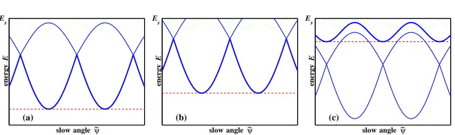
Fig. 1 Schematic figure illustrating the formation of the peak of the function∆Esm(−)(ωf): (a)ωf=

ωmax; (b)ωf<ωmax; (c)ωf>ωmax. The relevant (lower) GSS curve is shown by the dotted

line. The relevant trajectories of the resonance Hamiltonian are shown by solid lines. The lower boundary of the layer is marked by a thick solid line: in (a) and (b) the lower boundary is formed by the lower part of the resonance separatrix while, in (c) it is formed by the resonance trajectory tangent to the GSS curve. The dashed line marks, for a givenωf, the maximal deviation of the

lower boundary from the separatrix energyEs.

35, 43, 44]), and the angle ˜ψmay take any value either from the range[0,π]or from the range[π,2π]5_.

After that, because of the closeness ofωf to then-th harmonic ofω(E)in the

relevant range ofE6_{, for a relatively long time the system follows the nonlinear} resonance(NR) dynamics (see Eq. (16) below), during the first half of which the deviation of the energy from the separatrix value grows, greatly exceeding δ for most of the trajectory. As time passes, ˜ψis moving and, at some point, the growth of the deviation changes for the decrease. This decrease lasts until the system hits the GSS curve, after which it returns to the separatrix just for one step of the separatrix map. At the separatrix, the slow angle ˜ψ changes random-like, so that a new stage of evolution similar to the one just described occurs, i.e. the nonlinear resonance dynamics starting from the GSS curve with a new (random) value of ˜ψ.

Of course, the SM cannot describe the variation of the energy during the velocity pulses (i.e. in between instants relevant to the SM): in some cases this variation can be comparable to the change within the SM dynamics. This additional variation will be taken into account below, where relevant.

One might argue that, even for the instants relevant to the SM, the SM describes the original Hamiltonian dynamics only approximately [31] and may therefore miss some fine details of the motion: for example, the above picture does not include small windows of stability on the separatrix itself. However these fine details are irrelevant in the present context, in particular the relative portion of the windows of stability on the separatrix apparently vanishes in the asymptotic limith→0.

5_{Of these two intervals, the relevant one is that in which the derivative dE/dtin the nonlinear}

resonance equations (see Eq. (16) below) is positive or negative, for the case of the upper or lower GSS curve respectively.

6_{I.e.Edetermined by Eq. (7) for any ˜ψexcept from the vicinity of multiples ofπ. As shown in}

The boundary of the SM chaotic layer is formed by those parts of the SM chaotic trajectory which deviate from the separatrix more than others. It follows from the structure of the chaotic trajectory described above that the upper/lower boundary of the SM chaotic layer is formed in one of the two following ways [43, 44]: (i) if there exists aself-intersectingresonance trajectory (in other words, the resonance separatrix) the lower/upper part of which (i.e. the part situated below/above the self-intersection) touches or intersects the upper/lower GSS curve while the up-per/lower part does not, then the upup-per/lower boundary of the layer is formed by the upper/lower part of this self-intersecting trajectory (Figs. 1(a) and 1(b)); (ii) oth-erwise the boundary is formed by the resonance trajectorytangentto the GSS curve (Fig. 1(c)). It is shown below that, in both cases, the variation of the energy along the resonance trajectory is larger than the separatrix split δ by a logarithmically large factor ∝ln(1/h). Therefore, over the boundary of the SM chaotic layer the largest deviation of the energy from the separatrix value,∆Esm(±), may be taken, in

the leading-order approximation, to be equal to the largest variation of the energy along the resonance trajectory forming the boundary, while the latter trajectory can be entirely described within the resonance Hamiltonian formalism.

Finally, we mention that, as is obvious from the above description of the bound-ary,∆Esm(±)≡∆Esm(±)(ωf)possesses a local maximum∆Emax(±),smatωf for which the

resonance separatrix justtouchesthe corresponding GSS curve (see Fig. 1(a)).

3 Single-Separatrix Chaotic Layer

It is clear from Sec. 2 above that∆Emax(±),sm is equal in leading order to the width

∆ENRof the nonlinear resonance which touches the separatrix. In Sec. 3.1 below,

weroughlyestimate∆ENRin order to classify two different types of systems. Secs.

3.2 and 3.3 present theaccurateleading-order asymptotic theory for the two types of systems. Thenext-ordercorrection is estimated in Sec. 3.4, while adiscussionis presented in Sec. 3.5.

3.1 Rough estimates. Classification of systems.

Let us roughly estimate∆ENR: it will turn out that it is thus possible to classify all

systems into two different types. With this aim, we expand the perturbationV into two Fourier series intand inψrespectively:

V ≡1

2

∑

(l)_(E,ψ)e−ilωft_+c.c.≡1

2

∑

(l)

As in standard nonlinear resonance theory [10, 23, 55, 51, 52], we single out the relevant (for a given peak) numbersKandLfor the blind indiceskandlrespectively, and denote the absolute value ofV_K(L)asV0:

V0(E)≡ |VK(L)(E)|. (9)

To estimate the width of the resonance roughly, we use the pendulum approxi-mation of resonance dynamics [10, 23, 55, 51, 52, 1]:

∆ENR∼ q

8hV0ωf/|dω/dE|. (10)

This approximation assumes constancy of dω/dEin the resonance range of ener-gies, which is not the case here: in reality,ω(E)∝1/ln(1/|E−Es|)in the vicinity of

the separatrix [53, 10, 23, 55, 51, 52, 1, 29, 34, 47, 35, 43, 44], so that the relevant derivative |dω/dE| ∼(ωr(±))2/(ω0|E−Es|)varies strongly within the resonance

range. However, for our rough estimate we may use the maximal value of|E−Es|,

which is approximately equal to∆ENR. Ifωf is of the order ofωr(±)∼ω0/ln(1/h), then Eq. (10) reduces to the following approximate asymptotic equation for∆ENR:

∆ENR∼V0(E=Es±∆ENR)hln(1/h), h→0. (11)

The asymptotic solution of Eq. (11) depends onV0(Es±∆ENR)as a function of

∆ENR. In this context, all systems can be divided in two types.

I The separatrix of the unperturbed system hastwo or moresaddles while the rele-vant Fourier coefficientV(L)_≡V(L)_{(E,ψ)possessesdifferentvalues on adjacent}

saddles. Given that, forE→Es, the system stays most of time near one of the

saddles, the coefficientV(L)_(E→E

s,ψ)as a function of ψ is nearly a “square

wave”: it oscillates between the values at the different saddles. The relevantK is typically odd and, therefore,V0(E→Es)approaches a well defined non-zero

value. Thus, the quantityV0(E=Es±∆ENR)in Eq. (11) may be approximated

by this non-zero limit, and we conclude therefore that

∆ENR∝hln(1/h), h→0. (12)

II Either (i) the separatrix of the unperturbed system has asingle saddle, or (ii) it has more than one saddle but the perturbation coefficientV(L)_{isidenticalfor all}

saddles. ThenV(L)_(E→E

s,ψ), as a periodic function ofψ, significantly differs

from its value at the saddle(s) only during a small part of the period inψ: this part is∼ω(E)/ω0∼1/ln(1/|Es−E|). Hence,V0(Es±∆ENR)∝1/ln(1/∆ENR).

Substituting this value in Eq. (11), we conclude that

∆ENR∝h, h→0. (13)

As shown below, the variation of energy in between the instants relevant to the SM is∼h, i.e. much less than∆ENR(12) for systems of the type I, and of the same

order as∆ENR(13) for systems of type II. Therefore, one may expect that the

max-imum width of the layer for the original Hamiltonian system (1),∆E(±)_{, is at least}

roughly approximated by that for the SM,∆Esm(±), so that the above classification of

systems is relevant to∆E(±) _{too. This is confirmed both by numerical integration}

of the equations of motion of the original Hamiltonian system and by the accurate theory presented in the next two sub-sections.

3.2 Asymptotic theory for systems of type I.

For the sake of clarity, we consider a particular example of a type I system; its generalization is straightforward.

We choose an archetypal example: the ac-driven pendulum (sometimes referred to as a pendulum subject to a dipole time-periodic perturbation) [55, 42, 45]:

H=H0+hV, (14)

H0= p2

2 −cos(q), V=−qcos(ωft), h¿1.

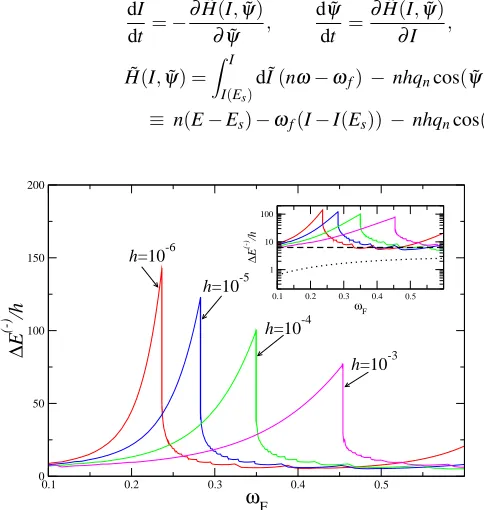
Fig. 2 presents the results of numerical simulations for a few values ofh and several values ofωf. It shows that: (i) the function∆E(−)(ωf)indeed possesses

sharp peaks whose heights greatly exceed the estimates by the heuristic [55], adia-batic [14] and moderate-frequency [29] theories (see inset); (ii) as predicted by our rough estimates of Sec. 3.1, the 1st peak of∆E(−)_(ω

f)shifts to smaller values of

ωf while its magnitude grows, ash decreases. Below, we develop a leading-order

asymptotic theory, in which the parameter of smallness is 1/ln(1/h), and compare it with results of the simulations.

Before moving on, we note that the SM (approximated in the relevant case by nonlinear resonance dynamics) considers states of the system only at discrete in-stants. Apart from the variation of energy within the SM dynamics, a variation of energy in the Hamiltonian system also occurs in between the instants relevant to the SM. Given thatωf ¿1, this latter variation may be considered in adiabatic

approxi-mation and it is of the order ofh[14, 35]. It follows from the above rough estimates, and from the more accurate consideration below, that the variation of energy within the SM dynamics for systems of type I is logarithmically larger i.e. larger by the factor ln(1/h). The variation of energy in between the instants relevant to the SM may therefore be neglected to leading-order for systems of type I:∆E(−)_'∆E(−)

sm .

For the sake of notational compactness, we shall henceforth omit the subscript “sm” in this subsection.

ω(E)' π

ln(32/|Es−E|), (15)

Es=1, |Es−E| ¿1.

Let us consider the range of energies belowEs (the range above Es may be

con-sidered in an analogous way) and assume that ωf is close to an odd multiple of

ωr(−). The nonlinear resonance dynamics of the slow variables in the range of

approximately resonant energies may be described as follows [43, 41] (cf. also [10, 23, 55, 51, 52, 1]):

dI dt =−

∂H(I˜ ,ψ)˜ ∂ψ˜ ,

d ˜ψ dt =

∂H(I˜ ,ψ)˜

∂I , (16)

˜

H(I,ψ˜) = Z _I

I(Es)

d ˜I(nω−ωf)−nhqncos(ψ˜)

≡ n(E−Es)−ωf(I−I(Es))−nhqncos(ψ)˜ ,

0.1 0.2 0.3 0.4 0.5

ω_F 0

50 100 150 200

∆

E

(-) /h

h=10-3 h=10-4

h=10-5 h=10-6

0.1 0.2 0.3 0.4 0.5 ω_F 1

10 100

∆

E

(-)/h

Fig. 2 Computer simulations for the ac driven pendulum (14) (an archetypal example of type I):

the deviation∆E(−)_{of the lower boundary of the chaotic layer from the separatrix, normalized by} the perturbation amplitudeh, is plotted as a function of the perturbation frequencyωf, for

vari-oush. The inset presents the same data but with a logarithmic ordinate and with the estimates by the heuristic [55], adiabatic [14] and moderate-frequency [29] theories. The heuristic estimate is shown by the dotted line: as an example of the heuristic estimate, we use the formula from [55]: ∆E(−)_/h=2πω

f/cosh(πωf/2). The adiabatic and moderate-frequency estimates are shown by

the dashed line: the adiabatic estimate for∆E(−)_(ω

f)is equal approximately to 2π; the estimate

following from the results of the work [29] forωf∼1 is of the same order, so that it is

I≡I(E) = Z _E

Emin

d ˜E

ω(E)˜ , E≡H0(p,q), ˜

ψ=nψ−ωft,

ψ=π+sign(p)ω(E) Z _q

qmin(E)

d ˜q

p

2(E−U(q))˜ +2πl,

qn≡qn(E) =_2π1 Z _2π

0 dψq(E,ψ)cos(nψ),

|nω−ωf| ¿ω, n≡2j−1, j=1,2,3, . . . ,

whereIandψare the canonical variables action and angle respectively [10, 23, 55, 51, 52, 1];Emin is the minimal energy over allq,p,E≡H0(p,q);qmin(E)is the minimum coordinate of the conservative motion with a given value of energyE;lis the number of right turning points in the trajectory[q(τ)]of the conservative motion with energyEand given initial state(q0,p0).

The resonance Hamiltonian ˜H(I,ψ˜)is obtained in the following way. First, the original Hamiltonian H is transformed to action-angle variablesI−ψ. Then it is multiplied bynand the termωfIis extracted (the latter two operations correspond

to the transformationψ→ψ˜≡nψ−ωft). Finally, the result is being averaged over

time i.e. only the resonance term in the double Fourier expansion of the perturbation is kept (it may be done since the effect of the fast-oscillating terms on the dynamics of slow variables is small: see the estimate of the corrections in Sec. 3.4 below).

Let us derive asymptotic expression forI(E), substituting the asymptotic expres-sion (15) forω(E)into the definition ofI(E)(16) and carrying out the integration:

I(E)'I(Es)−Es_π−E µ

ln

µ

32 Es−E

¶

+1

¶

. (17)

As for the asymptotic valueqn(E→Es), it can be seen thatq(E→Es,ψ), as a

function ofψ, asymptotically approaches a “square wave”, oscillating between−π andπ, so that, for sufficiently smallj,

q2j−1(E→Es)'(−1)j+1 2

2j−1, (18)

q2j=0,

j=1,2, ...¿ π

2ω(E).

The next issue is the analysis of the phase space of the resonant Hamiltonian (16). Substituting ˜H(16) into the equations of motion (16), it can be seen that their stationary points have the following values of the slow angle

˜

ψ+=π, ψ˜−=0, (19)

nω−ωf∓nhdqn

dI =0, n≡2j−1, (20) where the sign “∓”corresponds to ˜ψ∓(19).

The term∝hin (20) may be neglected to leading-order (cf. [10, 23, 55, 51, 52, 1, 43, 41]), and Eq. (20) reduces to the resonance condition

(2j−1)ω(Er(j)) =ωf, (21)

the lowest-order solution of which is

Es−Er(j)'32 exp µ

−(2j−1)π ωf

¶

. (22)

Eqs. (19) and (22) together with (17) explicitly determine the elliptic and hyper-bolic points of the Hamiltonian (16). The hyperhyper-bolic point is often referred to as a “saddle” and corresponds to ˜ψ+or ˜ψ−in (19) for even or odd jrespectively. The

saddle point generates the resonance separatrix. Using the asymptotic relations (17) and (18), we find that the resonance Hamiltonian (16) takes the following asymp-totic value in the saddle:

˜

Hsaddle'Es−E (j) r

π ωf−2h

'ωf π 32 exp

µ

−π(2j−1) ωf

¶

−2h. (23)

The second asymptotic equality in (23) takes into account the relation (22). As explained in Sec. 2 above,∆E(−)_(ω

f)possesses a local maximum atωf for

which the resonance separatrix is tangent to the lower GSS curve (Fig. 1(a)). For the relevant frequency rangeωf →0, the separatrix split (which represents the

maxi-mum deviation of the energy along the GSS curve fromEs) approaches the following

value [55] in the asymptotic limith→0

δ'2πh, ωf ¿1. (24)

As shown below, the variation of energy along the relevant resonance trajectories is much larger. Therefore, in the leading-order approximation, the GSS curve may simply be replaced by the separatrix of the unperturbed system i.e. by the horizontal lineE=Esor, equivalently,I=I(Es). Then the tangency occurs at ˜ψ, shifted from

the saddle byπ, so that the condition of tangency is written as

˜

Hsaddle=H(I˜ =I(Es),ψ˜=ψ˜saddle+π)≡2h. (25)

Substituting here ˜Hsaddle (23), we finally obtain the following transcendental

xexp(x) =8(2j−1)

h , x≡

(2j−1)π ωmax(j)

. (26)

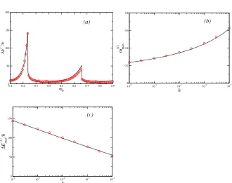
Fig. 3(b) demonstrates the excellent agreement between Eq. (26) and simulations of the Hamiltonian system over a wide range ofh.

In the asymptotic limith→0, the lowest-order explicit solution of Eq. (26) is

ωmax(j) ' (2j−1)π ln

³

8(2j−1) h

´, j=1,2, ...¿ln

µ

1 h

¶

. (27)

As follows from Eq. (26), the value ofEs−Er(j)(22) forωf=ωmax(j) is

Es−Er(j)(ωf =ωmax(j)) = 4πh ωmax(j)

. (28)

Its leading-order expression is:

0.1 0.2 0.3 0.4 0.5 0.6 0.7 0.8 0.9

ωF 0

50 100 150 200

∆

E

(-)/h

(a)

10-6 ₁₀-5 ₁₀-4

10-3 10-2

h

0 0.2 0.4 0.6 0.8

ωmax

(1)

0

(b)

10-6 ₁₀-5 ₁₀-4 ₁₀-3 ₁₀-2

h

0 50 100 150

∆

Emax

(1)

/h

(c)

Fig. 3 An archetypal example of a type I system: the ac-driven pendulum (14). Comparison of

the-ory (solid lines) and simulations (circles) for: (a) the deviation∆E(−)_(ω

f)of the lower boundary

of the chaotic layer from the separatrix, normalized by the perturbation amplitudeh, as a function of the perturbation frequencyωf, forh=10−6; the theory is from Eqs. (26), (31), (32), (38), (39)

and (41) (note the discontinuous drop by the factor e from the maximum to the right wing). (b) The frequency of the 1st maximum in∆E(−)_(ω

f)as a function ofh; the theory is from Eq. (26).

(c) The 1st maximum in∆E(−)_(ω

Es−Er(j)(ωf =ωmax(j))'_2j4h₋₁ln

µ

8(2j−1) h

¶

, h→0. (29)

Ifωf ≤ωmax(j) then, in the chaotic layer, the largest deviation of energy from the separatrix value corresponds to the minimum energyE_min(j) on the nonlinear reso-nance separatrix (Fig. 1(a,b)), which occurs at ˜ψshifted byπfrom the saddle. The condition of equality of ˜Hat the saddle and at the minimum of the resonance sepa-ratrix is written as

˜

Hsaddle=H(I(E˜ min(j)),ψ˜saddle+π). (30)

Let us seek its asymptotic solution in the form

Es−E_min(j) ≡∆E_l(j)= (1+y)(Es−Er(j))'(1+y)32 exp µ

−π(2j−1) ωf

¶

,

y∼>1. (31)

Substituting (31) and (23) into Eq. (30), we obtain forythe following transcen-dental equation:

(1+y)ln(1+y)−y= h

8(2j−1)xfexp(xf), (32)

xf ≡π(2j−1)

ωf , ωf ≤ω (j)

max, y>0,

whereωmax(j) is given by Eq. (26).

Eqs. (31) and (32) describe the left wing of the j-th peak of∆E(−)_(ω

f). Fig. 3(a)

demonstrates the good agreement between our analytic theory and simulations for the Hamiltonian system.

It follows from Eq. (26) that Eq. (32) for ωf =ωmax(j) reduces to the relation ln(1+y) =1, i.e.

1+y(ωmax(j)) =e. (33)

It follows from Eqs. (33), (31) and (28) that the maximum for a given peak is:

∆Emax(j) ≡Es−E_min(j)(ωmax) =(j) 4πeh

ωmax(j)

. (34)

Fig. 3(c) shows the excellent agreement of this expression with our simulations of the Hamiltonian system over a wide range ofh.

The leading-order expression for∆Emax(j) is:

which confirms the rough estimate (12).

Asωf decreases, it follows from Eq. (32) thatyincreases exponentially sharply.

In order to understand how∆E_l(j)decreases upon decreasingωf, it is convenient to

rewrite Eq. (31) re-expressing the exponent by means of Eq. (32):

∆E_l(j)(ωf) =_ω 4πh

f(ln(1+y)−y/(1+y)). (36)

It follows from Eqs. (32) and (36) that∆E_l(j) decreasespower-law-likewhenωf is

decreased. In particular,∆E_l(j)∝1/(ωmax(j) −ωf)at the far part of the wing.

As for the right wing of the peak, i.e. forωf >ωmax(j), over the chaotic layer, the largest deviation of energy from the separatrix value corresponds to the minimum of the resonance trajectory tangent to the GSS curve (Fig. 1(c)). The value of ˜ψ at the minimum coincides with ˜ψsaddle. In the leading-order approximation, the GSS

curve may be replaced by the horizontal lineI=I(Es), so that the tangency occurs

at ˜ψ=ψ˜saddle+π. Then the energy at the minimumE_min(j) can be found from the

equation

˜

H(I(Es),ψ˜saddle+π) =H(I(E˜ min(j)),ψ˜saddle) (37)

Let us seek its asymptotic solution in the form

Es−Emin(j) ≡∆Er(j)=z(Es−Er(j))'z32 exp µ

−π(2j−1) ωf

¶

0<z<1, z∼1. (38)

Substituting (38) into (37), we obtain forzthe following transcendental equation:

z(1+ln(1/z)) = h

8(2j−1)xfexp(xf) (39)

xf ≡π(2_ωj−1)

f , ωf >ω

(j)

max, 0<z<1,

whereωmax(j) is given by Eq. (26). Eqs. (38) and (39) describe the right wing of the j-th peak of∆E(−)(ωf). Fig. 3(a) demonstrates the good agreement between our

analytic theory and simulations.

It follows from Eq. (26) that the solution of Eq. (39) forωf →ωmax(j) isz→1, so the right wing starts from the value given by Eq. (28) (or, approximately, by Eq. (29)). Expressing the exponent in (38) from (39), we obtain the following equation

∆Er(j)(ωf) =_ω 4πh

It follows from Eqs. (39) and (40) that∆Er(j)decreasespower-law-likefor

increas-ingωf. In particular,∆Er(j)∝1/(ωf−ωmax)(j) in the far part of the wing. Further

analysis of the asymptotic shape of the peak is presented in Sec. 3.5 below. Beyond the peaks, the function∆E(−)_(ω

f)is logarithmically small in

compari-son with the maxima of the peaks. The functions∆E_l(j)(ωf)and∆Er(j)(ωf)in the

ranges beyond the peaks are also logarithmically small. Hence, nearly any function of∆Er(j)(ωf)and∆E_l(j+1)(ωf)which is close to∆Er(j)(ωf)in the vicinity ofωmax(j) and to∆E_l(j+1)(ωf)in the vicinity ofωmax(j+1)while being sufficiently small beyond the peaks may be considered as an approximation of the function∆E(−)_(ω

f)to

log-arithmic accuracy with respect to the maxima of the peaks,∆Emax(j) and∆Emax(j+1), in the whole range[ωmax(j) ,ωmax(j+1)]. One of the easiest options is the following:

∆E(−)_(ω

f) =∆E_l(1)(ωf) for ωf <ωmax(1),

∆E(−)(ωf) =max{∆Er(j)(ωf),∆E_l(j+1)(ωf)} for ωmax(j) <ωf<ωmax(j+1),

j=1,2, ...¿ π

2ωmax(1)

. (41)

We used this function in Fig. 3(a), and the analogous one will also be used in the other cases.

In fact, the theory may be generalized in such a way that Eq. (41) would approxi-mate∆E(−)(ωf)well in the ranges far beyond the peaks with logarithmic accuracy,

even with respect to∆E(−)_(ω

f)itself rather than to∆Emax(j) only (cf. the next sec-tion). However, we do not do this in the present case, being interested primarily in the leading-order description of the peaks.

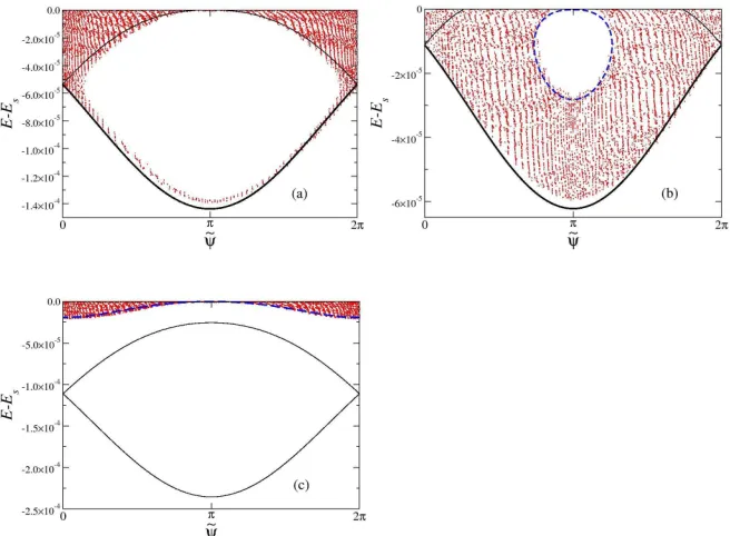
Finally, we demonstrate in Fig. 4 that the lowest-order theory describes the boundary of the layers quite well, even in the Poincar´e section rather than only in energy/action.

3.3 Asymptotic theory for systems of type II.

Fig. 4 Some characteristic Poincar´e sections in the 2π-interval of the energy-angle plane for the system (14) withh=10−6_andω

f equal to: (a) 0.236 (maximum), (b) 0.21 (left wing), (c) 0.25

(right wing). Results of the numerical integration of the equations of motion for the original Hamil-tonian (14) are shown by (red) dots. The NR separatrix calculated in the leading-order approxima-tion (i.e. by the integraapproxima-tion of the resonant equaapproxima-tions of moapproxima-tion (16) in whichω(E),I(E)and

q1(E)are approximated by the explicit formulæ (15), (17) and (18) respectively) is drawn by the

(black) solid line. The NR trajectory (calculated in the leading-order approximation) tangent to the lineE=Esis drawn by the (blue) dashed line. The outer boundary (marked by a thicker line) is

approximated by: the lower part of the NR separatrix in cases (a) and (b), and by the tangent NR trajectory in case (c) The boundary of the island of stability in the cases (a) and (b) is approximated by the tangent NR trajectory (which coincides in the case (a) with the NR separatrix).

3.3.1 AC-driven Duffing oscillator.

Consider the following archetypal Hamiltonian [1, 18, 29, 40]:

H=H0+hV, (42)

H0= p 2

2 − q2

2 + q4

4 , V=−qcos(ωft), h¿1.

ω(E)' 2π

ln(16/(Es−E)), (43)

Es=0, 0<Es−E¿1.

Correspondingly, the resonance values of energies (determined by the condition analogous to (21)) are

Es−Er(j)=16 exp µ

−2πj ωf

¶

, j=1,2,3, ... (44)

The asymptotic dependence ofI(E)is

I(E)'I(Es)−Es_2π−E µ

ln

µ

16 Es−E

¶

+1

¶

. (45)

The nonlinear resonance dynamics is described by the resonance Hamiltonian ˜H which is identical in form to Eq. (16). Obviously, the actual dependencesω(E)and I(E)are given by Eq. (43) and (45) respectively. The most important difference is inqj(E): instead of a non-zero value (see (18)), it approaches 0 asE→Es. Namely,

it is∝ω(E)[1, 13]:

qj(E)'√1

2ω(E), j=1,2, ...¿

π

ω(E), (46)

i.e.qjis much smaller than in systems of type I (cf. (18)). Due to this, the resonance

is “weaker”. At the same time, the separatrix splitδ is also smaller, namely∼hωf

(cf. [43]) rather than∼has for the systems of type I. That is why the separatrix chaotic layer is still dominated by resonance dynamics while the matching of the separatrix map and nonlinear resonance dynamics is still valid in the asymptotic limith→0 [43].

Similarly to the previous section, we find the value of ˜H in the saddle in the leading-order approximation7:

˜

Hsaddle'ωf Ã

Es−Er(j)

2π −

h √ 2

!

, (47)

whereEs−Er(j)is given in (44).

As before, the maximum width of the layer corresponds toωf, for which the

resonance separatrix is tangent to the GSS curve (Fig. 1(a)). It can be shown [43] that the angle of tangency asymptotically approaches ˜ψsaddle+π=πwhile the energy

still lies in the resonance range. Hereω(E)≈ωr(−)≈ωf/j. Using the expressions

for ˜H(E,ψ)˜ (cf. (16)), I(E) (45),qj(E)(46), and taking into account that in the

tangencyE<δ ∼hωf ¿h, to leading-order the value of ˜Hat the tangency reads

7_{The only essential difference is thatq}

nat the saddle is described by Eq. (46) rather than by Eq.

˜

Htangency'ωf√h

2. (48)

Allowing for Eqs. (47) and (48), the condition for the maximum, ˜Hsaddle=

˜

Htangency, reduces to

Es−Er(j)(ωmax(j))'2π √

2h. (49)

Thus these valuesEs−Er(j) are logarithmically smaller than the corresponding

values (28) for systems of type I.

The values ofωf corresponding to the maxima of the peaks in∆E(−)(ωf)are

readily obtained from (49) and (44):

ωmax(j) ' 2πj

ln(4√2/(πh)), j=1,2, ...¿ln(1/h). (50)

The derivation to leading order of the shape of the peaks for the chaotic layer of the separatrix map, i.e. within the nonlinear resonance (NR) approximation, is similar to that for type I. So, we present only the results, marking them with the subscript “NR”.

The left wing of the jth peak of∆E_NR(−)(ωf)is described by the function

∆E_l(_,NRj) (ωf) =16(1+y)exp µ

−2πj ωf

¶

≡ 2π

√ 2h

ln(1+y)−y/(1+y), (51) ωf≤ωmax(j),

whereyis the positive solution of the transcendental equation

(1+y)ln(1+y)−y= πh 4√2exp

µ

2πj ωf

¶

, y>0. (52)

In common with the type I case, 1+y(ωmax(j) ) =e, so that

∆E_max(j)_,NR=e(Es−Er(j)(ωmax))(j) '2πe √

2h. (53)

Eq. (53) confirms the rough estimate (13). The right wing of the peak is described by the function

∆E_r(_,j)_NR(ωf) =16zexp µ

−2πj ωf

¶

≡ 2π √

2h

1+ln(1/z), (54)

ωf >ωmax(j),

z(1+ln(1/z)) = πh 4√2exp

µ

2πj ωf

¶

, 0<z<1. (55)

As in the type I case,z(ωf→ωmax)(j) →1.

It follows from Eqs. (49) and (53) that the typical variation of energy within the nonlinear resonance dynamics (that approximates the separatrix map dynamics) is ∝h. For the Hamiltonian system, the variation of energy in between the dis-crete instants corresponding to the separatrix map [55, 51, 52, 1, 43, 31] is also ∝h. Therefore, unlike the type I case, one needs to take it into account even at the leading-order approximation. Let us consider the right well of the Duffing potential (the results for the left well are identical), and denote bytkthe instant at which the

energyE at a givenk-th step of the separatrix map is taken: it corresponds to the beginning of thek-th pulse of velocity [55, 43] i.e. the correspondingqis close to a left turning point qlt pin the trajectory [q(τ)]. Let us also take into account that

the relevant frequencies are small so that the adiabatic approximation may be used. Thus, the change of energy fromtkup to a given instanttduring the following pulse

of velocity (t−tk∼1) may be calculated as

∆E= Z _t

tk

dτqhcos(ω˙ fτ)'hcos(ωftk) Z _t

tk

dτq˙

=hcos(ωftk)(q(t)−qlt p) (56)

For the motion near the separatrix, the velocity pulse corresponds approximately toψ=0 (see the definition ofψ(16)). Thus, the corresponding slow angle is ˜ψ≡

jψ−ωftk' −ωftk.

For the left wing of the peak of ∆E(−)_(ω

f) (including also the maximum of

the peak), the boundary of the chaotic layer of the separatrix map is formed by the lower part of the NR separatrix. The minimum energy along this separatrix occurs at

˜

ψ=π. Taking this into account, and also noting that ˜ψ' −ωftk, we conclude that

cos(ωftk)' −1. So,∆E≤0, i.e. it does lower the minimum energy of the layer of

the Hamiltonian system. The maximum reduction occurs at the right turning point qrt p:

max(|∆E|)'h(qrt p−qlt p) = √

2h. (57)

We conclude that the left wing of the j-th peak is described as follows:

∆E_l(j)(ωf)'∆E_l(_,j)_NR(ωf) + √

2h, ωf ≤ωmax(j), (58)

where∆E_l(_,j)_NR(ωf) is given by Eqs. (51)-(52). In particular, the maximum of the

peak is:

∆Emax(j) '(2πe+1) √

2h≈25.6h. (59)

cos(ωftk)'1 and, hence,∆E ≥0. So, this variation cannot lower the minimum

energy of the layer for the main part of the wing, i.e. forωf ≤ω_bend(j) whereω_bend(j) is

defined by the condition∆E_r(_,NRj) =max(|∆E|)≡√2h. Forωf>ω_bend(j) , the minimal

energy in the layer occurs at ˜ψ=π, and it is determined exclusively by the variation of energy during the velocity pulse (the NR contribution is close to zero at such ˜ψ). Thus, we conclude that there is a bending of the wing atωf =ωbend(j) :

∆Er(j)(ωf) =∆Er(,NRj) (ωf), ωmax(j) <ωf ≤ωbend(j) ,

∆Er(j)(ωf) = √

2h, ωf ≥ω_bend(j) ,

ω_bend(j) = 2πj

ln(8√2/h) +1−2π, (60)

where∆E_r(_,j)_NR(ωf)is given by Eqs. (54) and (55).

Analogously to the previous case, ∆E(−)_(ω

f) may be approximated over the

whole frequency range by Eq. (41) with∆E_l(j) and∆Er(j) given by Eqs. (58) and

(60) respectively. Moreover, unlike the previous case, the theory also describes ac-curately the range far beyond the peaks:∆E(−) _{is dominated in this range by the}

velocity pulse contribution∆E, which is accurately taken into account both by Eqs. (58) and (60).

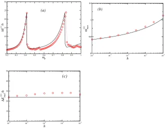
Fig. 5 shows very reasonable agreement between the theory and simulations, especially for the 1st peak8_.

3.3.2 Pendulum with an oscillating suspension point

Consider the archetypal Hamiltonian [1, 18, 29, 34, 35]

H=H0+hV,

H0= p 2

2 +cos(q), V =−cos(q)cos(ωft), h¿1. (61) Though the treatment is similar to that used in the previous case, there are also characteristic differences. One of them is the following: although the resonance Hamiltonian is similar to the Hamiltonian (16), instead of the Fourier component

8_{The disagreement between theory and simulations for the magnitude of the 2nd peak is about}

three times larger than that for the 1st peak, so that the height of the 2nd peak is about 30% smaller than that calculated from the asymptotic theory. This occurs because, for the energies relevant to the 2nd peak, the deviation from the separatrix is much higher than that for the 1st peak. Due to the latter, the Fourier coefficientq2(E)for the relevantEis significantly smaller than that obtained

of the coordinate,qn, there should be the Fourier component of cos(q),Vn, which

can be shown to be:

V2j'(−1)j+14

πω(E), Es−E¿1, (62)

V2j−1=0,

j=1,2, ...¿ 2π

ω(E), Vn≡ 1 2π

Z _2π

0 dψcos(q)cos(nψ).

The description of the chaotic layer of the separatrix map at the lowest order, i.e. within the NR approximation, is similar to that for the ac-driven Duffing oscillator. So we present only the results, marking them with the subscript “NR”.

The frequency of the maximum of a given j-th peak is:

0.2 0.3 0.4 0.5 0.6 0.7 0.8 0.9 1

ωF 0

5 10 15 20 25

∆

E

(-)

/h

(a)

10-6 ₁₀-5 ₁₀-4

10-3 10-2

h

0 0.5 1 1.5

ωmax

(1)

0 0.5 1 1.5

(b)

10-6 ₁₀-5 ₁₀-4 ₁₀-3 ₁₀-2

h

0 10 20 30 40 50

∆

Emax

(1)

/h

(c)

Fig. 5 An archetypal example of a type II system: the ac driven Duffing oscillator (42).

Com-parison of theory (solid lines) and simulations (circles): (a) the deviation∆E(−)_(ω

f)of the lower

boundary of the chaotic layer from the separatrix, normalized by the perturbation amplitudeh, as a function of the perturbation frequencyωf, forh=10−6; the theory is from Eqs. (41), (50), (51),

(52), (54), (55), (58) and (60) (note the discontinuous drop from the maximum to the right wing); (b) the frequency of the 1st maximum in∆E(−)_(ω

f)as a function ofh; the theory is from Eq. (50);

(c) the 1st maximum in∆E(−)_(ω

ωmax(j) ' 2πj

ln(4/h), j=1,2, ...¿ln(4/h). (63)

This expression agrees well with simulations for the Hamiltonian system (Fig. 6(b)). To logarithmic accuracy, Eq. (63) coincides with the formula following from Eq. (8) of [34] (reproduced in [35] as Eq. (21)) taken in the asymptotic limit h→0 (or, equivalently,ωmax(j) →0). However, the numerical factor in the argument of the logarithm in the asymptotic formula following from the result of [34, 35] is half our value: this is because the nonlinear resonance is approximated in [34, 35] by the conventional pendulum model which is not valid near the separatrix (cf. our Sec. 3.1 above).

The left wing of the jth peak of∆E_NR(−)(ωf)is described by the function

∆E_l(_,NRj) (ωf) =32(1+y)exp µ

−2πj ωf

¶

≡ 8h

ln(1+y)−y/(1+y), (64)

ωf≤ωmax(j),

whereyis the positive solution of the transcendental equation

(1+y)ln(1+y)−y=h 4exp

µ

2πj ωf

¶

, y>0. (65)

Similarly to the previous cases, 1+y(ωmax) =(j) e. Hence,

∆E_max(j)_,NR=e(Es−Er(j)(ωmax(j))) =8eh. (66) Eq. (66) confirms the rough estimate (13). The right wing of the peak is described by the function

∆E_r(_,j)_NR(ωf) =32zexp µ

−2πj ωf

¶

≡ 8h

1+ln(1/z), (67) ωf >ωmax(j),

wherez<1 is the solution of the transcendental equation

z(1+ln(1/z)) =h 4exp

µ

2πj ωf

¶

, 0<z<1. (68)

Similarly to the previous cases,z(ωf →ωmax)(j) →1.

close to−π/2 orπ/2 respectively. So, let us calculate the change of energy from the beginning of the pulse,tk, until a given instanttwithin the pulse:

∆E=− Z _t

tk

dτqh∂V˙ /∂q=h Z _t

tk

dτq(˙ −sin(q)cos(ωfτ))

'hcos(ωftk) Z _t

tk

dτq(˙ −sin(q))'hcos(ωftk)(cos(q(t))−1). (69)

Here, the third equality assumes adiabaticity while the last equality takes into ac-count that the turning points are close to the maxima of the potential i.e. close to a multiple of 2π (where the cosine is equal to 1).

The quantity∆E (69) takes its maximal absolute value atq=π. So, we shall further consider

∆Emax=−2hcos(ωftk)≡ −2hcos(2jψk−ψ˜k) = (−1)j+12hcos(ψ˜k). (70)

The last equality takes into account that, as mentioned above, the relevant ψk is

either−π/2 orπ/2. For the left wing, the value of ˜ψat which the chaotic layer of the separatrix map possesses a minimal energy corresponds to the minimum of the resonance separatrix. It is equal toπ or 0 if the Fourier coefficientV2jis positive or

negative, i.e. for odd or even j, respectively: see Eq. (63). Thus∆Emax=−2hfor any jand, therefore, it does lower the minimal energy of the boundary. We conclude that

∆E_l(j)(ωf)'∆E_l(_,NRj) (ωf) +2h, ωf ≤ωmax(j) , (71)

where∆E_l(_,j)_NR(ωf) is given by Eqs. (64)-(65). In particular, the maximum of the

peak is:

∆Emax(j) '(4e+1)2h≈23.7h. (72)

The expression (72) confirms the rough estimate (13) and agrees well with sim-ulations (Fig. 6(c)). At the same time, it differs from the formula which can be ob-tained from Eq. (10) of [34] (using also Eqs. (1), (3), (8), (9) of [34]) in the asymp-totic limith→0: the latter gives for∆Emax(j) the asymptotic value 32h. Though this result [34] (referred to also in [35]) provides for the correct functional dependence onh, it is quantitatively incorrect because (i) it is based on the pendulum approxi-mation of the nonlinear resonance while this approxiapproxi-mation is invalid in the vicinity of the separatrix (see the discussion of this issue in Sec. 3.1 above), and (ii) it does not take into account the variation of energy during the velocity pulse.

The right wing, by analogy to the case of the Duffing oscillator, possesses a bend atωf =ωbend(j) where∆E

(j)

∆Er(j)(ωf) =∆Er(,NRj) (ωf), ωmax(j) <ωf ≤ω_bend(j) ,

∆Er(j)(ωf) =2h, ωf ≥ω_bend(j) ,

ω_bend(j) = 2πj

ln(16/h)−3, (73)

where∆E_r(_,j)_NR(ωf)is given by Eqs. (66) and (67).

Similarly to the previous case, both the peaks and the frequency ranges far be-yond the peaks are well approximated by Eq. (41), with∆E_l(j) and∆Er(j)given by

Eqs. (71) and (73) respectively (Fig. 6(a)).

0.2 0.3 0.4 0.5 0.6 0.7 0.8 0.9 1

ω_F

0 5 10 15 20 25 30

∆

E

(-)

/h

(a)

10-6 10-5 10-4 10-3 10-2

h

0 0.5 1 1.5

ωmax

(1)

0 0.5 1 1.5

(b)

10-6 10-5 10-4 10-3 10-2

h

0 10 20 30 40 50

∆

Emax

(1)

/h

(c)

Fig. 6 An archetypal example of a type II system: the pendulum with an oscillating

suspen-sion point (61). Comparison of theory (solid lines) and simulations (circles): (a) The deviation ∆E(−)_(ω

f)of the lower boundary of the chaotic layer from the separatrix, normalized by the

per-turbation amplitudeh, as a function of the perturbation frequencyωf, forh=10−6; the theory

is by Eqs. (41), (63), (64), (65), (67), (68), (71) and (73) (note the discontinuous drop from the maximum to the right wing). (b) The frequency of the 1st maximum in∆E(−)_(ω

f)as a function of h; the theory is from Eq. (63). (c) The 1st maximum in∆E(−)_(ω

f)/has a function ofh; the theory