Transfer operators for deterministic and stochastic coupled map lattices

(1)

A Thesis Submitted for the Degree of PhD at the University of Warwick

Permanent WRAP URL:

http://wrap.warwick.ac.uk/88630

Copyright and reuse:

This thesis is made available online and is protected by original copyright. Please scroll down to view the document itself.

Please refer to the repository record for this item for information to help you to cite it. Our policy information is available from the repository home page.

(2)

Transfer Operators for

Deterministic and Stochastic

Coupled Map Lattices

Torsten Fischer

Thesis submitted for the degree of

Doctor of Philosophy at the University of Warwick

..

Mathematics Institute

University of Warwick

Coventry

(3)

List of Figures

1.1 h-line and r-line . . . . . . . 1. 2 2-triangle . . . .

1.3 Consecutive r-line and h-line . . . 1.4 Combination 2-triangle and h-line .. 1.5 Example for a configuration . . .

1.6 The labelled graph for the configuration in Figure 1.5

13 14 14 15 17 29

2.1 The history of qo . . . . 61

2.2 A reduced configuration 82

2.3 A full configuration . . . 82 '

(5)

Acknowledgements

I would like to express my gratitude to my supervisor Hans Henrik Rugh for his great support throughout my Ph.D. studies. He introduced me to the theory of transfer operators and coupled map lattices. I enjoyed our long discussions about mathematics and other things in a friendly atmosphere and his help in raising a scholarship for me.

I am grateful to Roger Tribe for his interest in my work and his enthusiasm in general. He initiated my work on the second part of my thesis and helped me in many discussions.

My thanks are also to Viviane Baldi, Torsten Hefer and Robert Reid for their help with the first part of my thesis and the participants of the weekly Ergodic Theory Seminar at the University of Warwick who provide a stimulating environment for working on dynamical systems.

I owe special thanks to my parents for their support and encouragement.

I was honoured to receive generous financial support via the the TMR-Fellowship ERBFMBICT-961157 and thank the EC.

Declaration

This thesis is composed of two chapters. Each chapter is written as an independent paper with its own introduction and notation. Chapter Two uses some results from Chapter One and refers to it by citation of the corresponding paper. The numbers in these citations refer to the numbering in Chapter One.

The paper constituting Chapter One has been accepted for publication in Ergodic Theory fj Dynamical Systems and is based on joint work with Hans Henrik Rugh.

It is not possible to distinguish exactly the individual contributions. However, each of us contributed a genuine part of proving the results.

(6)

Summary

In Chapter One we consider analytically coupled circle maps (uniformly expand-ing and analytic) on the Zd-Iattice with exponentially decayexpand-ing interaction. We introduce Banach spaces for the infinite-dimensional system that include measures whose finite-dimensional marginals have analytic, exponentially bounded densities. Using residue calculus and 'cluster expansion'-like techniques we define transfer op-erators on these Banach spaces. We get a unique (in the considered Banach spaces) probability measure that exhibits exponential decay of correlations.

(7)

Chapter

1 Transfer Operators for Coupled

Analytic Maps

1.0 Introduction

Coupled map lattices were introduced by K. Kaneko (cr. [20] for a review) as systems that are mixing wrt. spatio-temporal shifts. L.A. Bunimovich and Ya.G. Sinai proved in [7] (cf. also the remarks on that in [4]) the existence of an invariant measure and its exponential decay of correlations for a one-dimensional lattice of weakly coupled maps by constructing a Markov partition and relating the system to a two-dimensional spin system.

JBricmont and A. Kupiainen extend this result in [3] and [4, 5] to coupled circle maps over the Zd-Iattice with analytic and Holder-continuous weak interaction, re-spectively. They use a 'polymer' or 'cluster'-expansion for the Perron-Frobenius operator for the finite-dimensional subsystems over A C Zd and write the nth

iter-ate of this operator applied to the constant function 1 in terms of potentials for a

d

+

I-dimensional spin system. Taking the limit as n ~ 00 and A ~ Zd they get existence and uniqueness (among measures with certain properties) of the invariant probability measure and exponential decay of correlations.

V. Baladi, M. Degli Esposti, S. Isola, E. Jarvenpaa and A. Kupiainen define in [1], for infinite-dimensional systems over the Zd lattice, transfer operators on a Frechet space, and, for d

=

1, on a Banach space; they study the spectral properties of these operators, viewing the coupled operator as a perturbation of the uncoupled one in the Banach case.

(8)

Coupled map lattices with multi-dimensional local systems of hyperbolic type have been studied by Ya.B. Pesin and Ya.G. Sinai [27], M. Jiang [16, 17], M. Jiang and A. Mazel [18], M. Jiang and Ya.B. Pesin [19] and D.L. Volevich [31, 32].

Detailed surveys on coupled map lattices can be found in [6], [19] and [4].

In the above papers (except [1], [21]) the analysis has been done only for Banach spaces defined for finite subsets A of the lattice, and the (weak) limit of the invariant measure for A -+ Zd was taken afterwards.

Here we present a new point of view in which a natural Banach space and transfer operators are defined for the infinite lattice of weakly coupled analytic maps (Section 1.1). The space contains consistent families of analytic densities over finite subsets of Zd. We take a weighted sup-norm so that the sup-norms of the densities for the sub-systems over finitely many (say N) lattice points is bounded exponentially in N

(Section 1.2). We identify an ample subset of this space with a set of rea measures

(Section 1.4) that contains the unique invariant probability density (Section 1.2). We derive exponential decay of correlations for this measure and a certain class of observables from (the proof of) the spectral properties of our transfer operators. (Sections 1.2, 1.7). The operator for the coupled system and also the invariant measure are (for a small interaction) in fact perturbations of their counterparts in the uncoupled case. So the mixing properties are inherited from the single site systems. Section 1.8 contains the proofs.

Our approach provides a natural setting for an analysis of the full Zd Perron-Frobenius operator in terms of cluster expansions .over finite subsets of the lat-tice. Using residue calculus we introduce an integral representation for the Perron-Frobenius operator for finite-dimensional sub-systems (Section 1.3) which yields a uniform control over the perturbation and also gives rise to an easy approach to stochastic perturbation (cf. [26]) which however we do not consider here.

Our 'cluster expansion' combinatorics (Section 1.5) uses ideas from the work of C. Maes A. Van Moffaert [26] who have introduced a simplified (compared to the one in [3]) polymer expansion. Apart from the analysis of the one-dimensional operator, which is fairly standard and for which we refer to e.g. [3], the paper should be self-contained.

1.1 General Setting

We consider coupled map lattices in the following setting: The state space is M =

(SI)Zd where SI = {z

Eel Izl

=

I}

is the unit circle in the complex plane and dE N.

The map S : M -+ M is the composition S = F 0 Tt of a coupling map Tt

(9)

Assumption I F(z)

=

(fP(ZP))PEZd where JP : SI -+ SI are real analytic and expanding (Le.

J;

~ Ao

>

1) maps that extend for some 151 holomorphically to the interior of an annulus A01 def

{z

Eel -15₁~ In

Izl

~

t5d

and the family of Perron-Frobenius operators C/p for the single site systems satisfies uniformly a condition

specified in Section (1.5.1) below (1.31). (We need some more definitions to specify these conditions. But note that they are in particular satisfied if all JP are the same.)

We write Tt: : M -+ M asTt:(z)

=

(T;(z))PEzd and T;(z)

=

zpexp[27ri€9p(Z)] with 9p(Z) = E~l 9p,k(Z). The function 9p,k is real valued on (Sl)Zd and depends only on

those Zq with lip - qll ~ k (neighbours of distance at most k) where IIpII def Et=l Ipd. We write Bk(p)

=

{q E Zd

I

lip - qll ~ k} and also denote by 9p,k the function from the finite-dimensional torus (SI )BJc(p) to R

We assume the following for the functions 9p,k:

Assumption II For all p E Zd and k ~ 1 each map 9p,k extends to a holomorphic map 9p,k : AZJc(p) -+ C and its sup-norm (of modulus) is exponentially bounded by

(1.1)

with Cl

>

0 and C2 bigger than a certain constant specified in (1.100).

The parameter Cl is actually redundant as it is multiplied by E in the definition of

T;.

We also have exp( -C2kd) ~ exp( -e) exp( -c

₂

k.d) for c

_{2 .}

C2 -

e, e

>

0, i.e. for any E we can make the interaction small only by taking C2 large. But once we have chosen C2 large enough to guarantee the convergence of the infinite sums in our analysis we can consider perturbations of the uncoupled map depending on the parameter E only.

With the metric

d-y(x, y) def sup ,I/pll IIxp - ypII (1.2) PEZd

for 0

< , <

1 (M, d-y) is a compact metric space. Its topology is the product topology on (SI )Zd. The Borel a-algebra B on M is the same as the product

0'-algebra. F and Tt: are continuous and measurable. Let C(M) denote the space of real-valued continuous functions on (M, d-y) with the sup-norm and f.l the Lebesgue (product) measure on M.

(10)

1.2 Main Results

For finite A C Zd let H(At) be the space of continuous functions on the closed polyannulus At that are holomorphic on its interior and write 11 •

IIA

for the

sup-norm (of modulus) on H(A~). Let F be the set of all finite subsets (including 0) of Zd. We denote by 1l the vectorspace of all consistent families ifJ = (ifJ".)AEF of functions ifJA E H(A~). Consistency means 7rAl ifJAa

=

ifJAl for Al ~ A2 E F. We write J-L( ifJ)

~

ifJ0'

We want to define a norm on a (sufficiently large) subspace of 1l that should at least contain 'product densities' like h

=

(hAhEF with hA(Z)

=

TIpEA hp (zp) , where hp E H(AJp}) is the invariant probability density for the single system over

{p}

(cf. Section 1.5.1).

Because of (1.32) the sup-norm IIhA1IIAl does not grow faster than exponentially in

IAII.

Therefore we take a weighted sup-norm. For 0

<

tJ

<

1 we define

(1.4)

and set 1l-o def {ifJ E 1llllifJlI-o

<

oo}. Then (1l-o, 11 ·11-0) is a Banach space. In fact, if (ifJn)nEN is a Cauchy sequence in (1l-o, 11·11-0) then for each A E F the sequence

(ifJ~DnEN

is Cauchy in the Banach space

(H(A~), II'"A~)

and so converges to ifJA' Consistency of (ifJA)AEF follows from taking the limit (as n

-+

00) of 7rAlifJAa

=

ifJAl using the continuity of 7rAl for any Al ~ A2 E F. Analogously we define for A E F

the weighted norm on spaces 1lA,-o of consistent sub-families (ifJAJAl~A:

(1.5)

We get the same (topological) vector space as (H(A~),

II·IIA),

but the constants for the estimates of the norms are unbounded as

IAI

increases. .

For given Al ~ A2 E F and N E N we have a map,

7rAl 0 £~AaoTAa •• 07rAa : (1l-o, 11· 11-0)

-+

(1lAl,-o, 11 . !lAl,-o) , (1.6)

where C~AaoTAa •• is the Perron-Frobenius operator for the finite-dimensional system over A2 (cf. Section 1.3) with fixed boundary conditions (not included in the nota-tion). The following definition of transfer operators for the infinite system does not depend on the choice of the boundary conditions.

Theorem 1.2.1 For tJ, f sufficiently small, C2, No sufficiently big and any Al E F:

1. The limit

(11)

E L ((tlD' 11 . liD)' (tl'll,DN' 11 • IIAI,DN)) exists for suitably chosen 0

<

'!91 ~ ... ~ '!9 No

=

'!9 No+!

= ... =

'!9 and the family of these operators is uniformly (in AI)

bounded. This defines operators r/:'oT~

E L ((tlD' 11 . liD)' (tlDN' 11 . IIDN)) by (.c!J.oT<if» Al def 'lrAI 0 C!J.oT<if>·

In particular for N ~ No we have C!J.oT< E L (tlD'

II . liD)'

In the case of finite-range interaction we can define a linear map CFoT< on tl

in the same way, i.e. if r is the range of interaction we set for any Al E F

(1.8)

2. There is an F 0 Tt. -invariant, non-negative probability measure v*. It is unique

in the set of non-negative probability measures whose marginal densities can be identified with a v = (VAJAIEF E llD.

In L(tlD' 11· liD) the sequence (C!J.oT')N>N, _{_} ₀ converges exponentially fast:

IIC!J.oT< - J.£(')v*IIL«ll",II"'''))

~

C3fjN

for some C3

>

0 and 0

<

fj

<

1.

(1.9)

Remark 1) The relation between measures and elements of tl is explained in Section 1.4, in particular in (1.23).

2) A formula for v is given in (1.59).

For the invariant measure v we have exponential decay of correlations for spatio-temporal shifts on the system:

Let (el,"" ed) be a linearly-independent system of unit vectors in Zd. We define translations 'Tei(p) def p+ei for pE Zd and ('Tei(z))p def ZTe.(P) for Z E M.

In the following theorem we denote by 'T (acting on M fro~ the right) compositions

'T = 'TI 0 ••. 0 'Tm(T) and by IJ a composition of spatio-temporal shifts (on M): IJ = IJI 0 . . . 0 IJm(<T)+n(<T) with IJi E {S, 'Tell"" 'T_{ed }.} We denote by n(IJ) the number of factors S and by m(IJ) the number of spatial translations in this product. For a translation-invariant system, i.e. fp

=

f and gp(z)

=

gTe~l(p)('Tei (z)) for all p E Zd

and i

=

1, ... , d, the time-shift S commutes with the translations.

(12)

1. If g E C((SI)Al) and f E C((SI)A2) then

IfMdv* gf - (fM dv* g) (fM dv* f)1 ~ c4'!9-IA11-IA21I1glloollfllooKdist(Al,A2),

where dist(A_1,A_{2 ) def}min{llp - qll : pEAl, q E A2 }.

2. If g E C((SI)Al) and f E 11. nC((SI)A2) then

IL

dv* gOT 0 snf -

(L

dv* gOT) (fM dv* f) 1 (1.10)

~ C(AI' A2 , K)c~AlI+IA211IgllooIlJIIA2Km(r)ijn

with suitable Cs and ij as in Theorem 1.2.1.

3. If the system is translation-invariant and g, f are as in (2. ), then

IL

dv*goaf-

(L

dv*g)

(L

dv* f)1 (1.11)

<

C(Ab A_{2 ,}K)c~Ad+IA211IglloollfIIA2Km(q)ijn(q).

4.

If g, f E C(M) then

lim

I

r

dv* gOT 0 sn f -

(r

dv* gOT)

(r

dv* f)

I

=

O.

max{m(r),n}-+oo

J

M

J

M

J

M

(1.12)

5. If the system is translation-invariant and g, f E C(M) then

max{m(!~~(q)}-+oo

L

dv* g 0 a f =

(L

dv* g)

(L

dv* f) . (1.13)

Remarks: 1) Statement (5.) means that for a translation-invariant system v is

mixing wrt. spatio-temporal shifts. According to (3.), the decay of correlations for observables g and h as specified in (2.) is exponentially fast.

(13)

1.3 Finite-Dimensional Systems

We first consider 'finite-dimensional versions' of the maps F, Tt etc. Let ~ =

(~P)PEZd E M be a fixed configuration. For a finite subset A C Zd we define

TA,t : A~

--+

CA by

(1.14)

where ZA V ~AC E M agrees with ZA on its A-sites and with ~AC on its AC-sites.

We do not specify ~A C in the notation of TA,t. The restriction of F to A~ is denoted by FA.

With the following two propositions we ensure that for sufficiently small 8 and € (independent of A and ZAC), the image of A~ wrt. FA 0 TA,E contains a bigger

polyannulus (cf. [3]) and the image of the boundary, FA 0 TA,E ([}A~), has positive

distance from A~.

For A C Zd _{we have the metric dA on (SI)A defined by}

(1.15)

Proposition 1.3.1 For all C7 E (0,1), sufficiently small 8 and € (depending on C7), and arbitrary A E :F \ {0}, TA,E maps A~ biholomorphically onto its image and TA,t (A~) :::> A~6' i.e. the image contains a sufficiently thick polyannulus. Also

TA,E ([}A~)

n

A~6 =

0,

i. e. the image of the boundary (the same as the boundary of the image) does not intersect the smaller polyannulus.

Proposition 1.3.2 Let the expanding maps fp : SI

--+

SI satisfy Assumption I for some 81 and an expansion constant Ao and let 1

<

A

<

Ao. Then for all sufficiently

small 8 (0

<

8

<

80) and all finite A C Zd the map FA : A~

--+

CA is locally biholomorphic, A~6 C FA (A~), i.e. the image contains a thicker polyannulus, and furthermore all Z E A~6 have the same number of preimages. We also have A~6

n

FA ([}A~) =

0.

Combining Propositions 1.3.1 and 1.3.2 we have for fixed C7 (from Proposition 1.3.1) and (small) 8

FA 0 TA,t

(At)

:::> A~>.6 (1.16)

and

(1.17)

In particular, if we choose C7

>

t

there is a disc of radius (e7A - 1)8

>

0 around each point in A~ that is entirely contained in FA 0 TA,E (A~). We will need this for

Cauchy estimates. From now on we keep 8 fixed.

In the next proposition we establish a special representation of the Perron-Frobenius operator for our finite system with (SI)N

=

(SI)A, SE

=

FAoTA,E, 'I/J continuous (the proposition holds also for 'I/J E VX>(M)) and cP continuous on the closed polyannulus

(14)

Definition 1.3.1 Let

,x

be a measure on a metric space M (with the Borel

0"-algebra) and let S : M -4 M be a measurable map which is non-singular wrt.

,x

(Le. for all measurable A E M, ,x(A)

=

0 implies ,x(S-l(A))

=

0). The Perron-Frobenius operator Cs, acting on Ll(M), is defined via the equation

(1.18)

that, for given </> E Ll(M), must hold for all 'I/J E LOO(M). The existence and unique-ness of Cs</> E Ll (M) is equivalent by the Radon-Nikodym Theorem to the absolute continuity (wrt.

,x)

of the measure associated to the functional 'I/J t-+

fM

d,x 'I/J 0 S </>

(the functional here is restricted to continuous functions

'I/J),.

and this follows from the nonsingularity of S.

Remark Setting 'I/J

=

1 in (1.18) we get that Cs preserves the integral:

L

d,x Cs</> =

L

d,x </>. (1.19)

The normalized Lebesgue measure p, on SI is given by dp,(z) = 2dz.1 (this lifts wrt.

the map

t

-4 eit to the normalized Lebesgue measure ;; on [0, 21r)T

~nd

the product

measure p,A on (SI)A is given by

d P, A ( ) _ z - dz 1 def - - -

IT

cf,zp 1

(21ri)IAI z 21ri zp .

pEA

(1.20)

We also use dp,A(z) as a shorthand notation for the right-hand side of (1.20) for

z E A~.

The following representation of the Perron-Frobenius operator for finite-dimensional subsystems of our coupled map lattice by means of Cauchy kernels is essential for our analysis. Similar Cauchy kernels were used in [28].

Proposition 1.3.3 With FA and TA,f defined as above set Sf = FA 0 TA,f and let

S; be the projection onto its p-th component. Then the Perron-Frobenius-Operator (for SE), acting on </> E ?-lA, can be written in the following way:

CS<</>(W) =

f

dJ-tA(z)</>(z)

IT

(8

_E(

)1_

S;(z))

Jr

A _pEA _{p Z} _wp

(1.21)

(15)

1.4 Further Remarks on the

Infinite-Dimensional System

The subspace of complex-valued functions that depend only on finitely many vari-ables is dense in (C(M), 11 . 1100)' and each such function (say depending on ZA only) can be uniformly approximated by (the restriction of) functions in ll.(At). The dual space of C(M) is rea(M) (see e.g. [11]), the space of bounded, regular, count ably additive, complex-valued set functions on (M, B) where B is the Borel a-algebra. The norm on rea(M) is the total variation. For given {j, A we consider rea measures

whose marginals have densities 4>AI(Sl)A over (81_)A_{(restriction of}_4>A_to₍₈1_)A)_S.t.

4> = (4)A)AeF E 1l..". We remark that not every 4> E ll.-o with real-valued 4>AI(Sl)A corresponds to an element in rea(M) because its variation might not be bounded as

fA

dj.£AI4>AI might be unbounded with A. So we define for 4> E 1l.

114>lIvar def lim

1

dj.£AI4>AI. (1.22)

A-+Zd (Sl)A

We set ll.bv _def_{4> _E_{1l. :}_114>lIvar

_<

_{oo} and}_1l.':;' _def_ll.bv

_n

_ll.-o. _{In particular all}

real-analytic and non-negative 4> E 1l., i.e. 4>AI(Sl)A ~ 0 for all A E F, belong to this space.

We can view every 4> E ll.bv as an element of rea(M): For 9 E C(M) the net (gA)AE:F given by gA def 'lrA(g) converges uniformly to g. We set

4>(g) def = .lim

1 .

_dj.£AgA4>A. A-+Zd (Sl)A

The limit exists because for Al C A2

1J(Sl

1

)A1 dj.£A1gAl4>A1

-1

(Sl )A2 dj.£A2gA24>A21

=

11 dj.£A2 (gAl - gA2)4>A21

(Sl )A2

::; IIgA1 - gA211(Sl)A2114>lIvar

gets arbitrarily small as Al -+ Zd, i.e. the net has the Cauchy property. We further see

114>llvar - sup

1

dj.£AI4>AI AE:F (Sl)A

sup sup

r

dj.£Ag 4>A AE:F 9EC«Sl)A) J(Sl)A

1191100S1

sup 14>(g)l,

(1.23)

(1.24)

(16)

so 114>lIvar is in fact the total variation (the operator-norm, cf. [11]) of the corre-sponding linear functional on C (M).

Let 1l(F) def UAEF H(A~) be the subspace of functions depending on only finitely

many variables. We define the product gl4> E 1lD of gl E 1l(A~l) and 4> E 1lD by

(1.26)

Lemma 1.4.1 If gl E H(A~l), g2 E H(A~2), g E C(M) and 4> E 1lD the following holds

1. The product in (1.26) is well-defined and

IIgl4>IID

~

IIgII1Al'l9-IAtllI4>IID'

2. (glg2)4> = gl(g24».

3. g2 can be considered as an element of 1-£19 and the product ylg2 as defined in

(1.26) is the same as the usual product between functions on M.

4.

(gl4>)(g)

=

4>(glg) where (gl4» and 4> act as functionals in the sense of

(1.23).

5. 1l~v is also a module over the ring 1-£ (F), i. e. in particular

Ilgl4>IIvar ~

IIgIIIA1II<l>llvar.

1.5 Expansion of the Perron-Frobenius Operator

We split the integral kernel of the Perron-Frobenius operator for a finite-dimensional system. Recall that r;(z)

=

zp exp (27rif E%:1 gp,k(Z))

= zp n~1 exp(27rifgp,k(z)) and that Sp(z)

=

fp

0

r;(z).

If we consider only finite range interaction, say up to distance l, we have .

l

r;,l(Z) def zp exp(27rif

L

gp,k(Z)). (1.27)

k==1

For a finite-dimensional system (say on (SI )A2) with fixed boundary conditions we have a special representation of

.c

FA 2oTA2 ,. in terms of the integral kernel (Proposition

1.3.3).

(17)

The sum in the right hand side converges uniformly in z E

rA

and wp E Aa.

1.5.1 The Unperturbed Operator

The first summand in (1.28) is just the one which appears in the uncoupled system (Le. Tf.=o

=

id) and in this case each lattice site can be considered separately. We denote by C /p the restriction of the Perron-Frobenius operator to the Banach space of functions on SI that extend continuously on the closed annulus Aa and holomorphicallyon the interior Aa· 11· IIA.s denotes the uniform norm over Aa. The operator

has 1 as simple eigenvalue and the rest of its spectrum is contained in a disc around

o

of radius strictly smaller than 1. It splits into

C/p

=

Qp

+

Rp (1.29)

with

RpQp

=

QpRp

=

0 (1.30)

and

/lR;/lL('1i(A6),II' IIA6) $ Cr'TJ,n (1.31)

with C_r

>

0 , 0

< 1]

<

1. For proofs of these statements see e.g. [3].

Qp is the projection onto the one-dimensional eigenspace spanned by hp E 1i(Aa),

whose restriction to SI is positive and has integral IS1 dJ-t hp

=

1. We assume in Assumption I regarding the family (JP)PEZd that

(1.32)

and the exponential bound in (1.31) both hold uniformly in p. This is the case for example if the fp are uniformly close to each other as is shown using analytic perturbation theory.

C/p preserves the integral (cf. (1.19)) and so does Qp, as follows e.g. from

(1.29)-(1.31). Since

r

+ is homologous to SI we can write Qp as

(18)

where we have used that g is holomorphic in Aa and defined:

h (w z) def {hp(Wp) for zp E

r+

p P' P 0 for zp E

r _

(1.35)

The idempotency Q; = Qp results in the integral representation

1

_-2·2"dz; 1

1

_-2dz! _{· lhp wP'zp}1 ( 2)h (2 1) ( I)

-1

dz! 1 1 1

p zP'zp g zp - -2 ·lhp(wp,zp)g(zp).

r 7r~ zp r 7r~ zp r 7r~ zp (1.36)

Here and throughout the section the upper indices in

z!, z;

etc. refer to the temporal

and the lower ones to the spatial coordinate in the space-time lattice Z x Zd.

According to Proposition 1.3.3 the operator Rp can be written

with

1

rp(wp, zp)

=

!: ( ) _

Jp(zp) - hp (wp, zp). p z wp

Then equation (1.30) results in the integral representation

1.5.2 The Perturbed Operator

In view of (1.28) we set

(1.37)

(1.38)

(1.39)

(1.40)

def JP 0 r;,k_1 (z) - JP 0 r; k(Z) {3p,k(wp, z) = wp (Jp 0 r;,k_1 (z) - wp)(J

P 0

r;,~(z)

_ wp) (1.41)

This corresponds to the difference between the operators for systems with interaction of finite-range of order k and k - 1, respectively. Using (1.1) we have the estimate

l{3p,k(Wp,z)1 (1.42)

<

Iwpllfp 0 r;,k_1 (z) - wpl-1lJp 0 r;,k(Z) - wpl-1 x IJp 0 r;,k_1 (z) - JP 0 r;,k(Z)

I

<

(1

+

(5)lc7A -11-1Ic7A -11-111f;II{p}CIEexp(-c2kd)

<

CSE exp( -c2kd )

(19)

1.5.3 Time N Step

Now we want to estimate the norm of (1.6) or equivalently that of

(1.43)

C~A20TA2'f</J(ZO)

=

JrA2 dp,A2(Z-I) ... JrA2 dp,A2(Z-N) n;~-N

n

_PEA2 (1.44) x (hp (z;+l ,z;)

+

rp(z;+l , z;)

+

2:::1

,Bp,k(Z;+l, zt)) </J(z-N)

(cf. also the beginning of Section 1.3.)

Distributing the product we get infinitely many summands. In each factor there is for each -N ::£ m ::£ -1, p E A2 a choice between hp, rp and ,Bp,k (1 ::£ k

<

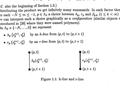
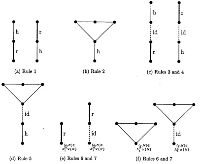
00) and we can interpret such a choice graphically as a configuration (similar objects were introduced in [26] where they were named polymers):

On A2 x {-N, ... , o} we represent

• hp (z;+l, z;) by an h-line from (p, t) to (p, t

+

1)

• r p (z;+l, z;) by an r-line from (p, t) to (p, t

+

1)

(p, t)

h (zHl zt) _{p p '}_p

(p,t+1)

(p, t)

r (zHl zt) _{P p ' p}

(p,t+1)

Figure 1.1: h-line and r-line

• ,Bp,k (z;+l, zt) by a k-triangle (actually rather a cone or pyramid but in our pictures for d

=

1 it is a triangle) with apex (p, t+1) and base points (q, t) with

lip - qll

::£ k. (So some of the base points might not lie in A2 x {-N, ... , -1} but all the apices lie in A2 x {-N

+

1, ... , o}.)

Note that if

(1.45)

denotes the number of base points of a k-triangle, we have the estimate v (k) ::£ (3k)d.

Each summand, that we get by distributing the product in (1.44), corresponds to a configuration and for each configuration C we have an operator Cc. So we can write

C~A20TA2"

=

2::

Cc.

c

[image:19.532.64.470.201.488.2]

(20)

(p - 2, t) (p - 1, t) (p, t) (p

+

1, t) - (p

+

2, t)

(p,t+1)

Figure 1.2: 2-triangle

• a factor h _{P p ' p}

(zH2

zHl)

r

_{P P ' p}(zHl

zt)

or

r (zH2

_{P P ' p}zHl) h (zHl _{P p ' p}

zt)

appears, but no factor ,Bq,k

(Z:+2,

zHl) with

I/p-ql/

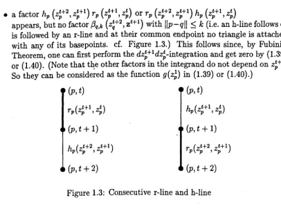
~ k (Le. an h-line follows or

is followed by an r-line and at their common endpoint no triangle is attached with any of its basepoints. cf. Figure 1.3.) This follows since, by Fubini's Theorem, one can first perform the dz;+ldz;-integration and get zero by (1.39) or (lAD). (Note that t~e other factors in the integrand do not depend on

z;+l.

So they can be considered as the function g(z;) in (1.39) or (lAD).)

(p, t) (p, t)

r

_{P p ' P}(zHl

zt)

h (zHl

zt)

P p ' p

(p,t+1) (p, t

+

1)

h

(zH2

zHl)

P p ' P

r (zH2

P p ' p zHl)

[image:20.530.136.409.44.155.2]

(p, t

+

2) (p, t

+

2)

Figure 1.3: Consecutive r-line and h-line

• if a term hp

(z;+2, z;+l)

,Bp,k

(z;+l ,zt)

appears but no ,Bq,l

(Z:+2,

zHl) with

lip - qll

~ l (Le. a triangle is followed by an h-line and at their common end point (the apex of the triangle) no other triangle is attached with any of its basepoints. Cf. Figure 1.4.) Indeed:

,Bp,k (wp, z) = wp

[1;

0

T~ ~z)

- w -

f

0

T~

\z) - w

1

p p,k P P p,k-l p

By the Residue Theorem:

1

dwp 1 ( )

- 2 . -,Bp,k W P' Z

=

0

SI 'lr1, Wp

(1.47)

[image:20.530.68.475.202.504.2]

(21)

because the poles at wp

=

JP

0 T:,k(~) and wp

=

JP

0 T:,k-I (z) (with z ErN,

in particular zp E

r

+ or

r -)

both he either outside

r

+ or inside

r -

as

JP

is expanding, T;,k is close to T;,k-I and the two summands have residue -1 and 1, respectively.

Identity (1.48) is a consequence of the fact that /3p,k is the kernel of a difference between two transfer operators (for the systems with interaction of range k

and k - 1) both preserving the Lebesgue integral in the sense of (1.19). So the range of this operator difference consists of functions with integral zero and these are annihilated by the operator corresponding to hp (cf. (1.33) and (1.34).)

(p, t)

h (zH2 zHI)

P p ' P

(p, t

+

2)

Figure 1.4: Combination 2-triangle and h-line

Furthermore we note that in

lI"A1 0 C:A20TA2,'

=

2:=

lI"A1 0 Cc

C

(1.49)

we get lI"A _oCc= 0 unless C ends with h-lines in all points of (A2 \ AI) x {O} because of (1.40),1(1.48) and the fact that lI"A1 means integration over (Sl)A2\A1.

Definition 1.5.1 We call a configuration Cc in the expansion (1.49) a zero configu-ration if it does not end with h-lines in all points of (A2 \ Ad x {O} or contains one of the constellations (consecutive r-line and h-line or k-triangle and h-line) mentioned above. Otherwise we call it a non-zero configuration.

Remark For a zero configuration C we have just shown that its corresponding summand in (1.49) is O. So we just have to sum over non-zero configurations. We note that the notion non-zero configuration does not exclude that .cc

=

O.

Ai;,

We have to find an upper bound for the norm of each Cc. We do so by collecting

(22)

Definition 1.5.2 • Let C be a non-zero configuration with exactly n{3,k

k-triangles for 1 ~ k

<

00. We define

and

def (

n{3 = n{3,b n{3,2, ••• )

00

In{31

def

L

n{3,k

<

00.

k=l

(1.50)

(1.51)

• A sequence ofh-linesfrom (p,t) to (p,t+1), ... , (p,t+k-1) to (p,t+k) with pE A2 and -N ~ t ~ t+k ~ 0 such that to the points (p, t+1) ... (p, t+k-1)

no triangles are attached is called an h-ehain of length k.

• If such an h-chain is not contained in a longer one it is called a maximal h-ehain. Then (p,

t)

and (p,

t

+

k) are denoted its endpoints.

• The definitions for a maximal r-ehain and its endpoints are analogous.

• Xc

denotes the set of points p E A2 that appear as the' Zd-coordinate of a ba~e point (p, t) of a triangle in C and

Ac

the set of those points p E Zd that appear

as the Zd-coordinate of an apex (p, t) that does not lie above (Le. having the same spatial coordinate) any other triangle.

• Ar is the set of pE Zd \

Ac

that appear as the Zd coordinate of an r-line (this

implies that there is an r-chain from (p, -N) to (p,O) for otherwise an r-line would have a common endpoint (p, t) with an h-line and C would be a zero configuration. )

def

-• We write A(C)

=

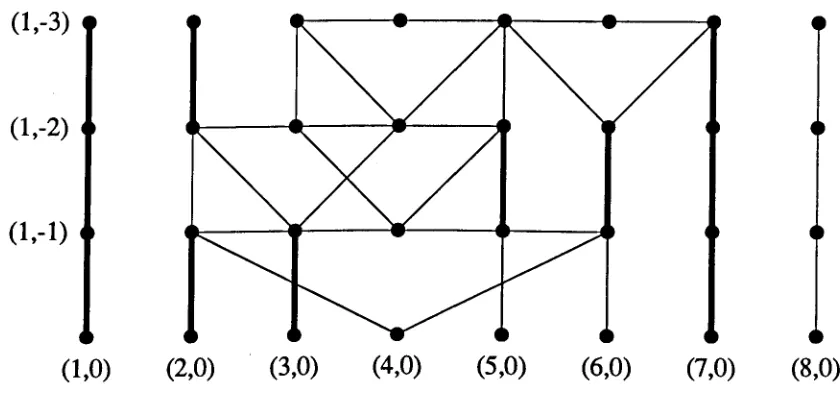
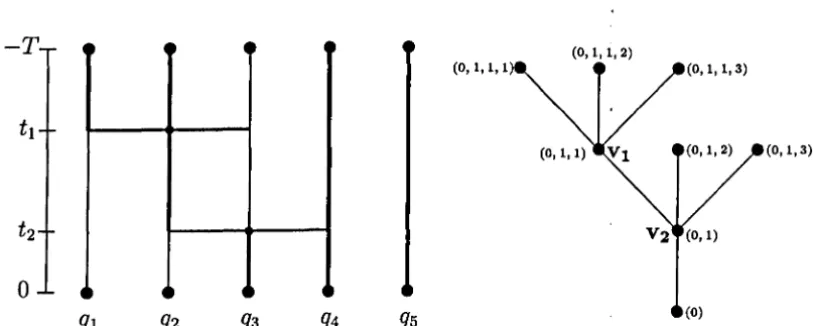
Ac U Ar •

In Figure 1.5 there are for example ~aximal r-chains from (1, -3) to (1,0) or from (2, -3) to (2, -2). A2 = {I, ... , 8},

Ac

=

{2, ... , 7},

Ac

=

{4} and Ar

=

{I}. As each k-triangle has v(k) ~ (3k)d base points we have

00

IAcl

~ I)3k)dn {3.k (1.52)

k=l

To get the estimate for the norm of (1.43) we proceed in the following order:

1. We integrate in I7rAl 0 Ccif> (z~J lover all dz; for which a factor

(23)

(1,-3)

(1,-2)

(1,-1)

[image:23.523.57.477.34.232.2]

(1,0) (2,0) (3,0) (4,0) (5,0) (6,0) (7,0) (8,0)

Figure 1.5: Example for a configuration

2. For each maximal h-chain starting at (p, t) and ending at (p, t

+

l) we perform the integration

3. We perform the integration corresponding to 7rAl

(1.54)

4. We estimate the contribution of each (from step 2 and 3 remaining) factor

hp(z;) by IIhpll_{Ao ::; Ch} and, using (1.42), the contribution of each factor

f3 (

p,k zHl zt) p , via

(1.55)

(24)

Remark For all points q

rt

Ac

U Ar we must have h-chains in C from (q, -N) to

(q,O). Therefore we have

(1.56)

where on the right-hand side we use the same notation 'Cc' for the operator on

Hil.cUAr/J·

So if n, denotes the number of r-lines,

nr

the number of maximal r-chains and

nh

the number of maximal h-chains having spatial coordinates in

Ac

U Al (for otherwise they are 'integrated away' giving a factor of 1) we get, using (1.31) and (1.55),

1/1I'Al 0 CCcPIIAl (1.57)

~

(csf)ln.s1 exp

(-C2

Ekdnp,k)

c:hc~"17n"IIcPAcUA,.IIil.cuA"

k=l

and, using (1.52),

(1.58)

00

<

'!9-IArl

n

'!9-(3~)dn.s,k 11 cPlI A2,11

k=I

for all

A2

E :F and with 11 • IIA2,11 defined in (1.5).

(1.57) and (1.58) are the basic estimates for a single configuration. We use refined versions of them throughout the paper.

In particular the idea of taking the norm of cP'AcUAr rather than that of cPA2 which grows with the size of A2 , is the key point in our analysis.

1.6 Operators for the Infinite-Dimensional

System

Estimates (1.57) and (1.58) bound the particular summands in an expansion like (1.49). We see that triangles and maximal r-chains in a configuration C lead to small factors on the right-hand side of (1.57). (A maximal r-chain consisting of n r-lines

contributes a factor cr17n• The factor er is greater than 1 in general. But either it

will be compensated for by a small factor due to a triangle e.g. as in (1.99) or n will

be large, cf. e.g. (1.103)). This motivates the following definition of the length of a configuration. The length gives rise to a lower bound for the number of triangles or r-lines, i.e. a long configuration will lead to a small contribution in the total sum in

(25)

Definition 1.6.1 • The length, length(C), of a non-zero configuration C (that we got in an expansion like (1.46)) is the maximal difference 0 - t such that there are points (p, t) and (q,O) being end-points of r-lines or base points or apices of triangles. (Note that if there are any triangles or r-lines, there is also a triangle or an r-line ending at A x {O}.) If there are no triangles or r-lines in C its length is zero.

• We identify two non-zero configurations Cl and C2 if they agree in their tri-angles, r-lines and their number of max h-chains that go upwards from base-points oftriangles (but might be defined on space-time boxes A2 x {-to, ... , O} of different sizes, i.e. with different A2 and to). We still speak of configurations rather than equivalence classes. For a configuration C length(C),

Ac,

A(C)

(as in the Definition 1.5.2) and the operator

7rA 0 Cc E L((1i(A~(C)), 11 'IIA(c)), (1i(At) , 11 • IIA)) is well-defined.

• For Al E F we define E(Ad as the set of all non-zero configurations C in some

A2 X {-to, ... , O} with Al C A2 E F, to E N and to

>

length(C), and that do not end in Al x {O} with triangles or r-lines.

• EN(Ad is the set of non-zero configurations C in A2 x {-N, ... , O} with Al C

A2 E F and A(C) ~ A2·

We define

VA def

L

7rA 0 CChA(C)' CEE(A)

(1.59)

The convergence of this infinite sum and other properties of v are stated in the

following proposition additional to Theorem 1.2.1.

Proposition 1.6.1 Let {), the sequence of {)i, f., C2, No and Al be as in Theorem

1.2.1 and N ~ No.

1.

7rAI 0 C1ftoT'

=

L

7rAI 0 Cc. (1.60) CEEN(AI)

2.

(1.61)

(26)

4·

For 1> E 1l': we have the estimate

(1.63)

For gEe (M) and 1> E 1l': we have the identity

(1.64)

and in particular

(1.65)

For finite-range interaction the inequality and both equations also hold for

1> E 1lbv•

5. CFoT< is non-negative, i.e. 1>

2::

0 implies CFoT<1>

2::

O.

(1)

>

0 means 1>A/(Sl)A

2::

o

for all A E F.)

1.7 Decay of Correlations

We have found the unique invariant v E 1£,0 with J.t(v) = 1. This corresponds to a non-negative measure on (M,8) whose marginal on (SI)A has density V/~Sl)A wrt.

J.tA• In the next theorem we state the decay of correlation for v in terms of the weighted norms. We will use these results in the proof of Theorem 1.2.2.

Theorem 1.7.1 For sufficiently small ~ and E, big~, finite disjoint AI, A2 and

f

E H(At2) there are a", E (0,1) and a {) E (0,1) such that

11 11

<

C ",dist(Al,A2)

1. VA1UA2 - VA1VA2 A1 UA2,t? _ 10 ,

2. I/1rAl(jV) - v(j)vA1IIA1,t?

S

cu{)-/A2/IIJIIA2",dist(Al,A2),

3. I/1rAl 0 C'JoT<(jv) - v(j)vA1IIA1,J

S

C12{)-/A21I/fI/A2",dist(A1,A2)fiN

for every N ~

o.

(27)

1.8 Proofs

In the proof of Proposition 1.3.1 we use the following lemma which is rather standard in real analysis. Here we formulate it in the setting of holomorphic functions.

Lemma 1.8.1 If T : U ~

en

is a holomorphic map on a convex set U

c

en

and satisfies the estimate I/DT(z) - idl/ :::; CIB

<

1 then T is biholomorphic onto its

image (in this lemma the chosen norm on

en

and the corresponding operator norm are both denoted by

/I .

I/J.

Proof T is locally biholomorphic by the Inverse Function Theorem. So we only have to show injectivity. Let zo,

ZI

E U with T (Zo)

=

T

(Zl)

and 'Y : [0, 1] ~ U ,

'Y(t) = Zo

+

t(Zl - Zo). Then

IlzI - z011

which implies

zl

= zO.

liT (Zl) - Zl -

T

(ZO)

+

z011

- liT

0 'Y(1) - 'Y(1) -

To

'Y(O)

+

'Y(O)

/I

- 1111

(DT (-y(t)) -,id)

(Zl -

ZO)

dtll

<

Ilzl - zOllll

I/DT(-y(t)) - idll dt

<

Ilzl - z011 ClB

(1.66)

o

Proof of Proposition 1.3.1 We have a Cauchy estimate for the partial derivatives of the functions gp,k : A:"'(p) ~ C on a smaller polyannulus. Let q E Bk(p), Then

1 d

<

I

6 £

I

Cl

exp( -C2k )

e - e"l

Also note that a~q gp,k = 0 for q ~ Bk (p). Therefore

00

<

C13

L

exp( -c2 kd )

k=llp-qll

, 1

<

C13

1 - exp ( ) -C2 exp (-c2I1p -

qlld)

(1.67)

(1.68)

(28)

Now we consider the lift given by pr : c~ --+ A~, (i'p)PEA t-+

(e

izp )PEA' where C_{6 def}{w E C

I

Imw E [-8, 8]} .

Then we have for the lifted functions (TA,f:

(z))

P

=

zp

+

27rf§p(Z). The function

gp(z) = gp(pr(z)) satisfies the same estimate (1.1) with a different constant

ci

for 8

<

81 sufficiently small since pr and its partial derivatives are uniformly bounded on C~.

Then we have

In particular the row sum norm (the operator-norm induced by the lOO-norm on CA)

of

(ny;;:;. -

id) is smaller than 1 for f

s~

enough, independent of A. According to Lemma 1.B.l (note that Cs is convex), TA,f: is a biholomorphic map onto its image and so is TA,E..

Now fix 8

<

81 according to the first part of the proof. If z E 8A~ we have zp E 8A6

for at least one pEA. From the formula z~ def T/'£(z)

=

zp exp (27rifgp(Z)) and the assumption that gp is uniformly bounded on A61 we see that

(1.70)

for sufficiently small f.

Now assume

0 f:.

AC76 \ TA,E. (A6) 3 z. Let s be the line-segment between z and its nearest point won (SI)A (wrt. the metric dA ). For each point y on s the inequality In dA(w, y) ~ In dA(W, z) ~ c178 holds.

In particular there is ayE TA,f: (8A~) on s with IYpl ~ c78 for all pEA, but this contradicts the estimate (1.70) above.

o

Proof of Proposition 1.3.2 As F acts on each coordinate separately by an

JP

we have (in view on the chosen metric (1.15)) to show the statement just for the map

J

(we drop the index p), i.e. the case when A contains just one element.

Consider the lift lRc; x R 3

(r,

</J) t-+

reit/J

where lRc; def [1 -In 8, 1

+

In 8]. This defines (modulo (0,27r) ) a (0, 27r)-periodic map

I

=

(IT! It/J)

via

J

(reit/J)

=

f,.(r, </J)eij",(r,t/J).

On {I}

x

R one has

!Ir

~ Ao and so because of periodic- . ity and a compactness argument,

!Ir

~ A on a thin (0

<

8

<

80 small) strip lRc; x Ht It follows similarly, as in the proof of Proposition 1.3.1, that

I

(lRc; x R) J RA6 X R,

I

is diffeomorphic onto its image and each point in lRc; x R has the same number of preimages (which is equal to (j(1,27r) -

j(1,

0)) /27r).

Fr~m

this the claim about

J

follows.

(29)

Proof of Proposition 1.3.3 We substitute the expression (1.21) into the right-hand side of equation (1.18) and get

r

dw 1

r

dz

rr (

1 S; (Z))

J(Sl)A (211"i)IAI W 'I/J(w) Jr A (211"i)IAI4>{z) pEA S;(z) - Wp Zp • (1.71)

To simplify notation we assume that A = {I, ... , N}. As (1.18) is linear in 'I/J we can assume (by using a continuous partition of unity) that 'I/J vanishes outside a small set K C {Sl)N having distinct preimages under

st

(for all 0 ~ t ~ €) contained in Ko

=

KOl X ••• x KON such that each Ko is contained in a polydisc Do

=

DOl X· •• x DON' These are mutually disjoint and

S~

def StDa is biholomorphic

onto its image (for all 0 ~ t ~ i). (To make this more precise we note that for

t

=

0 the map SO is the product of maps fi (1 ~ i ~ N) and each fi gives rise to an Mi-fold covering map of A6. So locally we can index the disjoint preimages of

K under SO by 0'

=

(a1,"" aN) where 1 ~ ai ~ Mi • If we take the set K small

enough this is still true under small (0 ~

t

~ €) perturbations.)

For given W E K, index a as above, k E {I, .. ;, N} and fixed Zl E A6_l (l

#-

k) the

function Zk H- (Sk(z!, ... , Zk,"', ZN) - Wk)-l has exactly one simple pole in each

Do,. and is holomorphic in A~ away from these poles. Therefore we get the same if

• 1

we Just integrate around these poles.

r

dw 1 ""

(rr

N

r

dZk)

rrN

$~

k{Z)

rrN

1 .

= J K (211"i)N

~'I/J(w) ~

k=l JaDa/o 211"i 4>(z) k=l

~k

k=l

S~Jk{Z)

- Wk' (1.72) For each a we can write each of the inner integrals as an integral of a differential form over the distinguished boundary boDo def aDol x '" x aD_{ON '} parameterized

by [0, I)N 3 t H- (e21ritl, ... , e21ritN) , whence

(1. 73)

We want to split the singular factor into a product of single poles in each variable. So we apply the transformation u = St{z) def S~(z) to get:

where (St-1)' is the complex derivative and so is holomorphic in u. To apply Cauchy's

(30)

homotopy between S£ and the product map So and avoids singularities of the inte-grand in (1.74) since for € small enough the set {St(boDo)J 0::;

t::;

€} has positive distance (uniformly in A) from the set of singularities Uk=I{U E Do : Uk = Wk}. So(boDo) = So,I(8Do

J

x ... x

So,N(8DoN ) is a product of cycles and hence a cycle. The differential n-form in (1.74) is a co cycle because its coefficient is holomorphic. So we get by Stokes' theorem

and by Cauchy's formula

-1( )rrN Wk 1

=

ljJ 0 S£ W k=1 (S;I(w))k

det(S~(S;l(w)))'

(1.76) So (1. 72) is equal to

~

1

dw 1 ( £) -1 ( ) 1 rrN Wk

~

K (27ri)N W 'Ij;(w)ljJ 0 So w

det(S£)'((S~)-I(w))

k=1

((S~)-I(w)h'

(1.77) For each index a, the coordinate transformation u = (S~)-I(w) yields

As 'Ij; 0 F = 0 outside Uo Ko and the Ko are mutually disjoint this equals

as was to be shown.

Proof of Lemma 1.4.1 Consistency follows from

7r Aa (glljJ) A4 7r Aa 0 7r A4 (glljJ Ai UA4) 7r Aa (glljJ Ai uA4 ) - 7r Aa (glljJ Ai UAa)

(glljJ) Aa

(1.78)

(1. 79)

(1.80)

o

(31)

for all A3 C A4 E :F.

As gl depends only on the AI-coordinates we have

and so

and

lI(glcl»AiUAIIAlUA - IIg1cl>AiuAII AlUA

<

IlllIAlllcl>AluAIIAluA

<

II g 1llAi -a-IAd-IAlllcI>IID

For Al fixed the product is continuous in both factors. (2.) follows from

((g lg2),I.)A 7r (gl g2 ,I. )

'I' - A Ai A2 'I' AuAi UA2

- 7r A (gt 7r AUAi (g~2 cl> AuAi UA2) )

- 7rA,(gt 7rAUAi (lcl>))

(gl(lcl»)A.

To see (3.) we note that the projection of the product of gl and g2 is

7rA(glg2) = 7rA(gtg~2)

and the product in the sense of (1.26) projects to

7rA(glg2)

=

7rA(gtg~uA2)

=

7rA(gtg~2)

as g2 does not depend on A \ A2-coordinates. If Al ~ A2 then

gA2(glcl»A2 gA2g1cl>A2 - (glg)A2c1>A2

and so (4.) follows from JZ;. .•

(1.82)

(1.83)

(1.84)

(1.85)

(1.86)

(1.87)

(32)

(5.) follows from

lim ( _dJlA2 9 A2 (gllfJ) A2 A2~Zd l(sl )A2

lim ( dJlA2 (glg)A2lfJA2

A2~Zd l(sl )A2

lfJ(glg)

lim { dJlA

I

(gllfJh

I

A~zdl(sl)A

lim ( dJlAlgllllfJAI

A-+zd l(sl)A A:>Al

<

IIgIIIA111lfJllvar

Proof of Lemma 1.5.1 We get recursively

(1.89)

(1.90)

o

f

0 Tt

~Z)

_ W JP 0 r;,I(Z) (1.91)

P p,l P

1

f

Tt () _ JP 0 r;,I_l(Z)

pO p,l-l Z wp

JP 0 r;,l-l (z) - JP 0 r;,I(Z)

The estimate (1.42) yields uniform convergence of this sum as l --+ 00. So we get (1.28).

o

(33)

Definition 1.8.1 • A maximal r-chain going from an apex of a triangle down-wards to the next basepoint of a triangle or to a bottom point is called an

a-r-chain. (If the apex coincides with a base or bottom point the a-r-chain has length zero.)

• The a-r-length of a configuration C is the sum of the lengths of all its a-r-chains plus the number of its triangles, i.e. if C has

Inpl

triangles with corresponding a-r-chains of length 1I, ... ,1lntll then

a-r-Iength(C) def 11

+ ... +

llntll

+

Inpl

(1.92)

- (11

+

1)

+ ... +

(llntll

+

1)

(In particular a-r-Iength(C) ~

Inpl·)

• We call a maximal r-chain going from a base point (p, t) of a triangle to (p, -N) (such that (p, -N) is not a base point of another triangle) a u-r-chain (upwards going r-chain), a maximal r-chain going downwards from a basepoint a

d-r-chain (d-h- d-r-chains are defined analogously).

• A maximal r-chain going from a bottom point (p,O) to (p, -N) is called an

l-r-chain (long r-chain). We denote the number of l-r-chains of C by l(C).

The configuration in Figure 1.5 has length 3, a-r-l~ngth 6, only one a-r-chain of positive length from (6, -2) to (6, -1), only one u-r-chain of positive length from (2, -3) to (2, -2), and only one l-r-chain from (1, -3) to (1,0).

We prepare the proofs of Theorem 1.2.1 and Proposition 1.6.1 in the following tech-nical proposition that provides the key bounds and basic analysis and combinatorics for the other proofs.

Proposition 1.8.1 For sufficiently small {), € and big C2 and N we have for all

Al ~ A2 E :F the following bound for the terms in the expansion of {1.49} for

'!rAl 0 £~A20TA2" with constants C19, C20:

1.

(1.93)

. th -def r.n

<

1 Wl 'f/

=

v'f/

2.

(34)

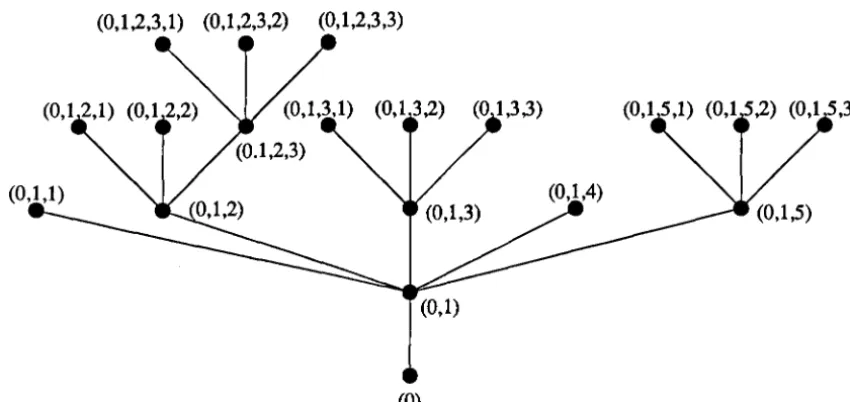
For the proof of Proposition 1.8.1 we need a graph-theoretical lemma. We consider labelled tree graphs that are constructed in the following way (cf. Figure 1.6): We start with a star graph with a root-vertex, labelled (0), to which K edges are

attached, each connecting to one leaf. The leaves are labelled by (0,1), ... , (0, K).

Then we add successively star graphs (~ach of these has a certain finite number v(k)

of leaves. These numbers are defined In (1.45).) to the already built up tree: We

identify one of the leaves of the tree, say labelled by S = (Sb ... , sn), with the root

of the added star and label the new leaves by (SI"",Sm1)"",(Sb""Sn,v(k)).

In total we use besides the star graph with K leaves exactly n(J,k star graphs with

exactly v(k) leaves. We say the tree has parameters K and n(J = (n(J,I, n(J,2, ... )

We also introduce a linear order on the set of tuples (and so on the set of vertices of the labelled graph):

We say S = (st, ... ,sn)

-<

t = (tl, ... ,tm ) ifn

<

m and Si

=

ti for 1 ~ i ~ n or if

Si = ti (1 ~ i

<

k) and Sk

<

tk for some k.

Lemma 1.8.2 1. The number of labelled tree graphs with exactly n edges is not greater than 22n

2. Given K, n{3,b n(J,2, .... with K

+

2:::1 n(J,k

<

00.

The number of labelled tree graphs with parameters K and n(J is bounded from above by

4K

n:l

~:np,k _with

C2l

_{= 4}3d_•

Proof of Lemma 1.8.2 We first prove (1.) For every' labelled tree graph in question we can define a path starting and ending at the root point (0) and running through each edge exactly twice in the following way. From a (labelled) vertex t

=

(t_{b ••• ,}

t

_k)

we go to the next greater (wrt.

-<)

vertex where we haven't yet been (going up), or if

this is not possible (i.e. t is a leaf or we have already been at all vertices (tl, ... , tk+l)) back to (tl,.'" tk-d (going down). So we return to (0) after 2n steps. We encode the path in a word (al,"" a2n) with ai

=

1 if we go up in the ith step and ai = 0

otherwise. Obviously the labelled graph is uniquely determined by its word. (Note that not every word of length 2n with symbols '0' and '1' corresponds to such a

labelled graph. But the map between these two data is injective.) As there are 22n

words of length 2n with at most two different symbols this is also an upper bound

for the number of graphs in question, so (1.) is proved.

To see (2.) we note, using the estimate for v(k) that we got after (1.45), that the

number of edges in such a tree graph is not greater than K

+

2:::1

(3k)dn(J,k.

o

(35)

(i) We fix 0 ~ K ~ IAII and Aa ~ Al with IAal

=

K (so there are (I~I) possible choices for Aa) and want to estimate the number of configurations C such that

Ac

=

Aa. So let us consider such a configuration. We call the triangles whose apex lies at, or whose a-r-chain ends in, Aa x {O}, root triangles. We can assign to C

a graph of the type we consider in Lemma 1.8.2 as follows: We start with a star graph with a star point labelled (0) and K leaves, labelled (0,1), ... , (0, K). These leaves are in bijection with Aa x {O}. Now we "add successively for each I-triangle (cf. def. on page 13) in C a star graph with one star point and v(l) leaves (cf. def. of v(l) in (1.45)) to the graph and label the new vertices: If an l-triangle lies with its apex or ends with its a-r-chain on a basepoint of another triangle (for which we have already assigned a small tree) or on a point in Aa x {O} (this point is labelled say S

=

(SI, ... , Sn)) we add a smalll-tree to the graph by identifying its star point with S and label the v(l) new leaves in the graph (SI, ••• , sn, 1), ... ,(SI, ••• , Sn, v(I)). Since, for example, an apex could coincide with more than one other triangle's basepoint we use the linear order

-<

(defined on page 28) to define an order in our successive assignment of triangles to star graphs. We always choose the next triangle such that the corresponding star graph is attached to the smallest (wrt.

-<)

labelled leaf in the graph. This also defines a unique choice of the triangle and the leaf where we attach the star graph. So the position of triangles and the a-r-chains of

C are completely determined by the datum consisting of the corresponding labelled

graph and the lengths of its a-r-chains. Note that it is not the case that for every graph together with a choice of lengths for the particular a-r-chains there was a corresponding configuration.

For the configuration in Figure 1.5, for example, we get the labelled graph in Figure 1.6.

(0,1,2,3,1) (0,1,2,3,2) (0,1,2,3,3)

(01,3,3)

(0)

[image:35.529.54.479.440.641.2]

(36)

Let n{3,k be, as in Definition 1.5.2, the total number of k-triangles. The number of

graphs with parameters K and n{3 is bounded by 4K n~1 ~;nl3,/c (by Lemma 1.8.2).

As mentioned above we have for each of the In{31 a-r-chains a length 0 ::::; li

<

00. The a-r-Iength is

L

=

(it

+

1)

+ ... +

(llnl3l

+

1). (1.95) So L ~ In{3l. For a given n{3 with In{31 ~ 1 and L ~ 1 there are (I~I~I) different

choices of (ll, ... , Ilnl3l) that satisfy (1.95). For In{31

=

0 we have L

=

0 and the (unique) configuration without triangles or r-lines. So in any case the number of choices is bounded from above by (I~I)· The integration over these In{31 a-r-chains

leads to a factor

J

nl3l7]L in our estimates (cf. (1.57)) and each k-triangle contributes by (1.55) a factor Cg€ exp( -C2kd).

(ii)

There are choices between d-r-chains and d-h-chains in the configuration.

There are not more than L:~I (3k)dn {3,k base points for which we can choose between

a d-h-chain (giving factor Ch in our estimates) and a d-r-chain (giving factor at most

C_r7]). So the total sum over these combinations is bounded from above by

00

(Ch

+

_Cr7]) Ek'=l (3k)d n13,/c ::::;

IT

(exp(c22kd)r13,1c .

k=1

(iii) There are choices between u-r-chains and u-h-chains in the configuration. There are not more than L:~I (3k )dn {3,k basepoints .. To each of them we can attach

either a u-h-chain, giving a factor Ch, or a u-r-chain, giving a factor Cr7]rnax.{O,N-L} , because if N - L

>

0, such a u-r-chain cannot have length smaller than N - L, for

otherwise it would not end in A2 x {-N}. We get in total a factor not greater than

00

(Ch

+

Cr)Ek'=1(3k)d n13,1c =

IT

(exp(c23 kd

)r

13,1c . _(1.96)

k=1

(iv) There are choices left between l-h-chains and l-r-chains in (AI

\Ac)

x{ -N, ... , O},

giving factor Ch or Cr7]N respectively. Let 1 (0 ::::; 1 ::::; IAI \ Acl ::::; IAII - K) denote the number of l-r-chains in such a choice. For given 1 there are (IAi

)Acl) ::::;

(IA1~-K) different subsets

Ar

of Al \

Ac

of cardinality 1 (that corresponds to a particular choice of exactly 1 l-r-chains.) The configuration C is determined by all the choices mentioned up to now.

Consider now a C with length(C)

=

N. If N - L

>

0 then there must be at least one u-r-chain giving rise to an extra factor 7]rnax.{O,N-L} or an l-r-chain giving rise to a factor 7]n. To get (1.98) we split

7]rnax.{O,N-L}

or 7]N

ijrnax.{O,N -L} ijrnax.{O,N -L}

-N-N

Transfer operators for deterministic and stochastic coupled map lattices