Received Jan 29, 2016 / Accepted Aug 21, 2016
Editorial Académica Dragón Azteca (EDITADA.ORG)
Incorporation of decision-maker preferences in an interactive
evolutionary multi-objective algorithm using a multi-criteria sorting
Laura Cruz-Reyes
1, Eduardo Fernández
2, Patricia Sánchez
3 *, Claudia Gómez
11
Tecnológico Nacional de México: Instituto Tecnológico de Ciudad Madero, México,
Universidad Autónoma de Sinaloa, México,
3Tecnológico Nacional de México: Instituto
Tecnológico de Tijuana, México.
[email protected], [email protected], [email protected],
[email protected]
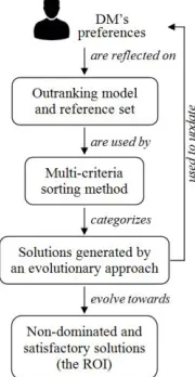
Abstract. Here, an interactive method is proposed to incorporate the preferences of the Decision Maker (DM) into the optimization process and lead the search towards the Region of Interest (ROI). The DM’s preferences are expressed in a reference set and are reflected by an outranking model. This information is used by a multi-criteria sorting method to create selective pressure towards solutions that are satisfactory to the DM. Our method obtains a better characterization of the ROI when compared with the well known NSGA-II and A2-NSGA-III in simple and complex project portfolio problems.
Keywords: Multi-Objective Evolutionary Algorithms, multi-criteria sorting, incorporation of preferences, interactive method.
1.
Introduction
A wide variety of problems in the real world involves several conflicting objectives to be optimized simultaneously under certain constraints [1].As a consequence of the conflicting nature of the criteria, there is no single solution that simultaneously optimizes each objective, so most approaches look for a set of trade-off solutions. This type of problem is known in the literature as the Multi-objective Optimization Problem (MOP). Solving MOPs means finding the compromise solution that best satisfies the preferences of the Decision Maker (DM) [2].
29
In this paper we propose a method, called the Interactive Multi-Criteria Sorting Genetic Algorithm (I-MCSGA), for incorporating the DM’s preferences interactively during the optimization process; the main contributions are summarized below. We propose to integrate the DM’s preferences with an MOEA in such a way that they can be incorporated implicitly and interactively in the evolutionary optimization algorithm. The preferences are modelled by an outranking paradigm, and also embedded in a reference set. A multi-criteria sorting method is used to identify new satisfactory solutions among those generated by the evolutionary search. These solutions are used i) to create selective pressure towards the ROI; and ii) to enhance the reference set in order to increase its assignment capacity. From time to time, the current satisfactory solutions are shown to the DM, who updates the reference set with them. In this way, the DM ‘learns’ progressively about the optimization problem, adjusts his/her (initially poorly defined) preferences, and then drives the search towards the ROI.
The rest of the paper is organized as follows. In Section 2 we give an overview of preference-based evolutionary methods, and we also describe a multi-criteria sorting method (the THESEUS method). With this background, an interactive approach for incorporating preference information, and the implementation of this approach, called I-MCSGA, are detailed in Section 3. In Section 4, we present computer experiments used to confirm the advantages of the proposed approach. Finally, some conclusions are discussed in Section 5.
2.
Background
2.1 A brief outline of preference-based evolutionary approaches
Multi-objective metaheuristic approaches have by now demonstrated their ability to approximate the whole Pareto front; however, the number of efficient solutions found is often too large. The selection of one solution (the final preferred alternative) from a huge set is evidently a difficult task for the DM, especially when the number of objectives increases [9]. As was mentioned above, because of humans’ cognitive limitations, as described by Miller [6],it is essential to provide the DM with a reduced number of satisfactory alternatives. The DM is only interested in discovering the zone of the Pareto front corresponding to his/her preferences (the ROI), rather than the whole Pareto front. Therefore, information about the DM’s preferences should be reflected by a representative model. The modelling of the preferences plays a key role in decision-making [10], since it will define the nature and organization of the information. The information about the DM’s preferences can be expressed in diverse ways. Bechikh [9]states that the preference information structures most commonly used are the following: weights (e.g. [11, 12]), ranking solutions (e.g. [13, 14]), ranking objectives (e.g. [15, 16]), reference point (e.g. [7, 17]), reservation point (e.g. [18]), trade-off between objectives (e.g. [19]), desirability thresholds (e.g. [20]) and outranking parameters (e.g. [2, 21]). The method in the recent paper of Oliveira et al. [22] lies in the last of these classes, because the preferences are expressed by an outranking relation and preference parameters. Oliveira et al. [22] use the ELECTRE TRI multi-criteria sorting method combined with an evolutionary algorithm. In ELECTRE TRI a reference profile is introduced to establish the boundary between two consecutive ordered categories. A critical aspect of ELECTRE TRI is defining the reference profiles because frequently is a very hard task for the DM, particularly when (s)he has just a vague conception regarding the boundary between adjacent categories. The existence of such boundaries is doubtful in many real-world problems (cf. [23, 24]). Besides, one can question whether a reference profile is sufficient for an acceptable characterization of the category related to it. If the object to be sorted were to be incomparable with several reference profiles, ELECTRE TRI would suggest inappropriate assignments.
The above approaches in evolutionary computation are grouped according to the different information structures used to incorporate the DM’s preferences. Another way of classifying these approaches depends on the stage at which the preference information is articulated by the DM. According to Hwang and Masud [25], preferences can be requested in several ways: a priori, a posteriori and interactively. A brief description of these is given below.
In an a priori approach, the DM’s preferences are articulated before the start of the method; the optimization process is then carried out by following the preference information. Afterwards, the optimization method finds the most-preferred point without additional interaction with the DM. However, the procedure is highly prone to error, since, unfortunately, the DM does not know how good is the best possible solution for the problem and how practical his/her aspirations are. Therefore, the DM may be dissatisfied with the outcome obtained. Some efforts in this direction can be found in [11, 26].
30
performs well in problems with few objectives, but the results deteriorate with an increase in the number of objective functions, as was discussed in the introduction to this paper. Some examples of a posteriori approaches are given in [27, 28].
The interactive approach depends on the progressive definition of the DM’s preferences, together with the exploration of the objective space. Articulation of preferences is performed during the optimization process, so that progress towards a particular region of the Pareto-optimal frontier is made. The DM must be willing to participate in the solution process and direct it according to his/her preferences. As the interactive process advances in identifying better solutions, the DM not only specifies his/her preferences, but also learns about the problem and can thus adjust his/her level of aspiration. Considering that the DM is part of the solution method, any solution in the set obtained has a high possibility of being accepted as the final solution. As stated by Hwang and Masud [25], some disadvantages of interactive methods are: (1) the solutions rely on the precision of the local preference that can be shown by the DM; (2) for several approaches there is no assurance that the most preferred solution can be achieved within a finite number of interactive steps; and (3) more effort is required of the DM than with the other methods presented above. There is a large variety of works in evolutionary multi-objective optimization that address the interactive approach (e.g. [29, 30]).
According to Miettinen et al. [31], interactive methods lessen the disadvantages of a priori and a posteriori methods because the DM can progressively refine his/her initial preferences, and only solutions that are interesting to the DM are generated. For this reason, we propose an interactive approach for obtaining a reduced set of efficient solutions adapted to the DM’s preferences. In addition, the approach of Fernandez et al. [2], the so-called NOSGA2, is an important precedent for our work. The a priori way of incorporating preferences in NOSGA2 has recently been used by Cruz et al. [32] to optimize interdependent project portfolios with many objectives. In that paper, the authors proposed the Non Outranked Ant Colony Optimization (NO-ACO) method that is briefly described below.
2.2 Description of the NO-ACO model
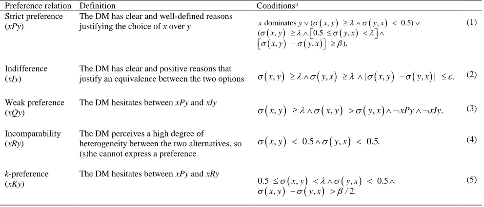
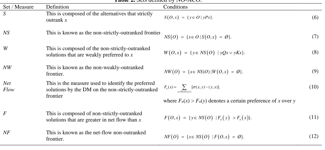
[image:3.612.50.546.478.691.2]The NO-ACO algorithm uses a set of agents called ants, and a local search, to perform its optimization process. This approach incorporates the DM’s preferences following the model of preferences by Fernandez et al. [2] that is based on outranking relations proposed by Roy in [33]. It uses the degree of truth of the statement ‘x is at least as good as y’, which is represented by σ (x, y), and can be calculated using outranking methods such as ELECTRE [34] and PROMETHEE [35]. Let us consider a threshold of acceptable credibility λ, an asymmetry parameter β to ensure the strict preference or k-preference, and a symmetry parameter ε for the indifference relation. For each pair of solutions (x, y), the model identifies one of the preference relations given in Table 1. Given a set of feasible solutions O, the preferential system of NO-ACO establishes the sets shown in Table 2.
Table 1. The preference relations between each pair of solutions.
Preference relation Definition Conditionsa
Strict preference (xPy)
The DM has clear and well-defined reasons
justifying the choice of x over y
dominates ( , , 0.5)
( , 0.5 ,
, , ).
x y x y y x
x y y x
x y y x
(1) Indifference (xIy)
The DM has clear and positive reasons that
justify an equivalence between the two options
x y,
y x, |
x y,
y x, | . (2)Weak preference (xQy)
The DM hesitates between xPy and xIy
x y,
x y,
y x, xPy xIy. (3)
Incomparability (xRy)
The DM perceives a high degree of
heterogeneity between the two alternatives, so (s)he cannot express a preference
x y, 0.5
y x, 0.5. (4)
k-preference (xKy)
The DM hesitates between xPy and xRy
0.5 , , 0.5
, , / 2.
x y y x
x y y x
(5)
31
Table 2. Sets defined by NO-ACO.
Set / Measure Definition Conditions
S This is composed of the alternatives that strictly
outrank x S O x , {yO yPx| }. (6)
NS This is known as the non-strictly-outranked frontier
{ | , }.
NS O xO S O x Ø (7)
W This is composed of the non-strictly-outranked
solutions that are weakly preferred to x W O x , {yNS O |yQxyKx}. (8)
NW This is known as the non-weakly-outranked
frontier. NW O {xNS O W O x( ) | , }.Ø (9)
Net Flow
This is the measure used to identify the preferred solutions by the DM on the non-strictly-outranked frontier
( )\{ }
( ) [ ( , ) ( , )].
n
y NS O x
F x x y y x
where Fn(x) > Fn(y) denotes a certain preference of x over y
(10)
F This is composed of non-strictly-outranked
solutions that are greater in net flow than x F O x , {yNS O |Fn y F xn }. (11)
NF This is known as the net-flow non-outranked
frontier. NF O {xNS O |F O x , }.Ø (12)
The problem that NO-ACO solves is
min
( , ) ,
( , ) ,
( , ) .
x O
S O x
W O x
F O x
(13) The best compromise solution is found through a lexicographic search, with pre-emptive priority favouring |S(O, x)|.2.3 An outline of the THESEUS method
Let us recall, following [36], some basic aspects of the THESEUS method. THESEUS employs outranking relations to solve multi-criteria sorting problems, where sorting refers to problems in which the categories have been defined in an ordinal way [37]. The aim of the THESEUS method is to assign multi-criteria objects to preference-ordered categories. THESEUS rests on the following premises (cf. [36, 38]):
i. There is a finite set of ordered categories Ct= {C1, …, CM}, (M ≥ 2); CM is assumed to be the preferred category.
ii. U is the universe of objects x described by a coherent set of N real-valued criteria, denoted G = {g1, g2, . . . , gj, . . . , gN},
with N ≥ 3.
iii. There is a set of reference objects T (also called a reference set or training set), which is composed of elements bkh ∈U
assigned to category Ck, (k = 1,..., M).
iv. The DM agrees with a fuzzy outranking relation σ (x, y) defined on U×U (see Section 2.2). Its value models the degree of credibility of the statement ‘x is at least as good as y’ from the DM’s perspective.
The THESEUS method is based on comparing a new object to be assigned with reference objects through models of preference and indifference relations (cf. [36]). The assignment is not a consequence of the object’s intrinsic properties: rather, it is the result of comparisons with other objects whose assignments are known. In the following, C(x) denotes a potential category for the assignment of object x. According to THESEUS, C(x) should satisfy some consistency rules:
,
khx U
b
T
,
. (14.a)
kh k
kh k
xPb C x C
b Px C C x · ·
,. (14.b)
kh k
kh k
xQb C x C
b Qx C C x · ·
( ) ( ). (14.c)
kh k k
k
xIb C x C C C x
C x C
32
The relations P, I, and Q were defined in Eqs. (1–3). The symbol ≿ denotes the statement ‘is at least as good as’ on the set of categories, which is related to the decision-making context. THESEUS uses the inconsistencies with Eqs. (14.a–c) to compare the possible assignments of x; more specifically:
The set of P-inconsistencies for x and C(x) is defined as DP = {(x,bkh), (bkh,x), bkh ∈ T such that (14.a) is FALSE};
The set of Q-inconsistencies for x and C(x) is defined as DQ = {(x,bkh), (bkh,x), bkh ∈ T such that (14.b) is FALSE};
The set of I-inconsistencies for x and C(x) is defined as DI = {(x,bkh), (bkh,x), bkh ∈ T such that (14.c) is FALSE}.
Suppose that C(x) = Ck and consider bjh∈ T. Some cases in which x and bjh belong to adjacent categories and nevertheless xIbjh may be explained by ‘discontinuity’ of the description; x may be close to the upper (lower) boundary of Ck and bjh may be close to the lower (upper) boundary of Cj. These are called second-order I-inconsistencies and are grouped in the set D2I. The set D1I = DI – D2I contains the so-called first-order I-inconsistencies, which are not consequences of the discontinuity effect described above. nP, nQ, n1I, and n2I denote the cardinalities of the inconsistency sets defined above. Let N1= nP + nQ + n1I, and N2 = n2I. THESEUS suggests an assignment that minimizes the above inconsistencies with lexicographic priority favouring N1, which is
considered the most important criterion [36]. The basic assignment rule is: For each x ∈ U and given a minimum credibility level λ > 0.5
i. Starting with k =1 (k =1,…,M) and considering each bkh∈ T, calculate N1 (Ck); ii. Identify the set {Cj} whose elements hold Cj = argmin N1 (Ck)
iii. Select Ck* = argmin N2(Ci); {Cj}
iv. Assign x to Ck*.
The suggestion may be a single category or a sequence of categories. The first case is called a ‘precise assignment’. Otherwise, the multi-category solution obtained highlights the highest category (CH) and the lowest category (CL); each category in this interval may be acceptable for the assignment of the object, but THESEUS fails to determine the most appropriate. A solution of this type is called an ‘imprecise assignment’.
According to recent studies by Fernandez et al. [38, 39], the capacity of THESEUS for suggesting appropriate assignments increases with the cardinality of the reference set. Fernandez et al. [38] proved that this capacity is improved with an automatic enhancement of the reference set, that is, when new objects are assigned by THESEUS and incorporated into the reference set without requiring acceptance by the DM.
3.
Our proposal
33
Fig. 1. The general scheme of the proposed approach to search the ROI.
3.1 An interactive approach to search the ROI based on a multi-criteria sorting method
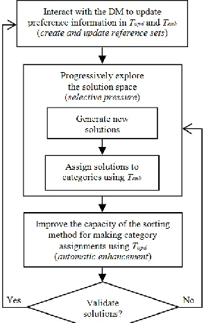
The proposal suggests using two reference sets, each one is divided into two categories: satisfactory and unsatisfactory. The first set, called Tupd, reflects the DM’s preferences that were obtained in the last interaction with him/her; the second one, called Tenh, accumulates new solutions through an automatic process. The two sets are identical at the beginning of the approach. The use of these sets and the description of the processes of our interactive approach are detailed below; Figure 2 illustrates these processes.
i. Interact with the DM to update preference information. This process aims to model the current DM’s preference
information, from his/her local knowledge. This information is represented by a set of solutions that the DM considers satisfactory or unsatisfactory, that is, a reference set (Tupd) that implicitly reflects his/her multi-criteria preferences. The interaction with the DM is performed at two points in time: a) at the beginning of the process, when Tupd is created with the first definition of the DM’s preferences; and b) during the search process, when Tupd is updated by the DM. The number of interactions will be limited by a given input parameter. The update can take place of the second interaction onwards and it is performed as set out below. First, the set Tenh is shown to the DM; Tenh contains new solutions categorized as satisfactory that is the result of an automatic enhancement process, which is described in (iii). The DM selects the solutions in that set that (s)he really considers satisfactory. Once the DM has performed this validation, the solutions in Tupd and Tenh must be replaced by the chosen solutions by the DM. The interaction allows the DM to learn, as new solutions are shown to him/her, and in this way (s)he adjusts his/her notion of what a satisfactory solution is. The update also allows the DM to correct possible errors of assignment that could be generated during the automatic enhancement procedure of Tenh. After each interaction, the reference set Tupd will contain the latest expression of the DM’s preferences. The validation of the preference information can be performed by a real DM or by an algorithm able to behave in a way that is similar to a real DM. It is important to highlight that the updating process is the essential part of this proposal, because by incorporating the DM into the solution approach, any of the solutions obtained at the end of the optimization process can be the solution to be implemented.
ii. Progressively explore the solution space. This process aims to create selective pressure towards the ROI, through an
exploration method that identifies, at least locally, new non-dominated solutions that would probably be considered as satisfactory by the DM. To perform this process two things are required: a) a procedure to guide the search towards efficient solutions in the sense of Pareto optimality; and b) an approach to capture the notion of a satisfactory solution. For the second of these, we consider it ideal to use a multi-criteria sorting method. This method will assign to predefined categories the new non-dominated solutions derived from the search process, using the preference information embedded in Tenh. This evaluation will help to direct selective pressure towards solutions assigned as satisfactory.
iii. Improve the capacity of the sorting method for making category assignments. This procedure aims to incorporate
34
Fig. 2. An interactive approach to search the ROI.
3.2 One way to specify the proposed approach: The Interactive Multi-Criteria Sorting Genetic Algorithm
Here, we present a way to implement the approach proposed in Section 3.1. This method, called the Interactive Multi-Criteria Sorting Genetic Algorithm (I-MCSGA), is based on the following points:
The DM’s preferences are reflected by an outranking model (x,y) built using ELECTRE III; this model contains a set of preference parameters (weights and thresholds of indifference, preference and veto). The DM’s preferences are also embedded in the reference set Tupd in which a set of solutions (actual or potential ones) are assigned by the DM as satisfactory and unsatisfactory. The set Tupd therefore contains the updated information about the DM’s preferences. The preference parameters in should be compatible with the preference information in Tupd. Such compatibility may be guaranteed (although this is not mandatory) by an indirect parameter elicitation method (e.g. [40]).
Since the ROI may be defined as a subset of the Pareto front whose elements are considered satisfactory by the DM, our method privileges (in a current population) solutions that are non-dominated and are considered satisfactory by a multi-criteria sorting method; in this work we use the THESEUS method. The way of creating selective pressure towards non-dominated solutions is inspired by the Non-dominated Sorting Genetic Algorithm-II (NSGA-II) [27], and is strengthened with the sorting of solutions.
The THESEUS method is used to make decisions on whether a particular solution in a current population is satisfactory or not. For making assignments, THESEUS uses the enhanced reference set Tenh. Before any enhancement Tenh Tupd. Tenh is automatically enhanced with new generated solutions that have been assigned to the satisfactory category by THESEUS using Tupd as reference set.
After a certain number of iterations, the satisfactory category of Tenh is presented to the DM, who updates Tupd with those solutions. The preference parameters may be updated from the current Tupd.
Remarks:
- As stated above, Tupd contains the most updated preferences from the real DM. Such an updating process is necessary for two main reasons: i) to correct the imprecise assignments made by the automatic enhancement of Tenh; and ii) because the DM ‘learns’ as (s)he ‘discovers’ new solutions and (s)he adjust his/her notion of what a satisfactory solution is.
35
- At the end of the search process, the satisfactory solutions of Tenh will be presented to the DM so that (s)he chooses the final solution from that set.
The general method of the I-MCSGA is shown in Algorithm 1. Note that it is composed of two main phases that will be described in the following subsections.
Algorithm 1. Procedure I-MCSGA
Input: L, num_iterations, enh_number, enh_interval, upd_number, upd_interval
Output: satisfactory category of Tenh Phase 1:
1. Construct an initial reference set Tupd //Section 3.2.1
2. Initialize Tenh with Tupd Phase 2:
3. Set σ-parameters agreeing with Tupd (using, for example, an indirect parameter
elicitation method)
4. Initialize parent population Pwith Tupd and complement it with random individuals
until a size L is achieved
5. Generate non-dominated fronts on P (based on objective function values)
6. Give to these fronts a rank (level) Fi according to non-domination level
7. Categorize the solutions in F1 using the THESEUS sorting method (σ) //Section 3.2.2
8. Generate a child population Qof size L by applying selection, recombination, and
mutation operators on P
9. FOR I=1 to num_iterations DO
10. P’ = P ∪ Q
11. Generate non-dominated fronts on P’ (based on objective function values)
12. Give to these fronts a rank (level) Fi according to non-domination level
13. Categorize the solutions in F1 using the THESEUS sorting method (σ) //Section 3.2.2
14. Create from P’ a new parent population P of size L by using a
diversity operator
//Section 3.2.3
15. Generate a child population Qof size L by applying selection, recombination,
and mutation operators on P
16. Enhance Tenh a certain number of times (enh_number) every certain
number of iterations (enh_interval)
//Section 3.2.4
17. Update Tupd (by interacting with the DM) a certain number of times
(upd_number) every certain number of iterations (upd_interval)
//Section 3.2.5
18. End FOR
19. Repeat steps 10−13 and 16
20. Give the DM the satisfactory solutions of Tenh
21. End PROCEDURE
3.2.1 A method to construct an initial reference set
In the first phase of the I-MCSGA, the DM is prompted to provide a reference set, which we call Tupd. The categories in that set are satisfactory and unsatisfactory. In order to create the reference set, the DM has the following two choices:
Provide a set of solutions in the objective space and, according to their objective values, indicate which of them are considered satisfactory, by using his/her current (limited) knowledge about the problem. These solutions do not necessarily have to be feasible, since they will only be used as a reference to start the search process. The DM may refine his/her aspiration levels during his/her interaction with the optimization process.
Run a multi-objective metaheuristic that matches the characteristics of the problem to be addressed. This approach will be used to obtain an approximation to the Pareto frontier. These solutions will be sorted by the DM into the set of categories to form the initial reference set. When this option is used to create the reference set, the method becomes a hybrid approach.
36
to Fernandez et al. [38], reference sets of large size should supply more knowledge about the assignment policy, leading to more appropriate assignments. Hence, in cases where the satisfactory category of the reference set is poorly populated, we recommend increasing the cardinality of this category. Therefore, we propose an approach for adding fictitious solutions (derived from an existing solution) to extend and intensify this category. The procedure to generate these solutions is as follows:
i. Identify a pair of objectives with nearly equal weights, called similar weight objectives; ii. Create a replica of an existing solution; and
iii. Modify the similar weight objectives of the replicated solution, adding to one of them and subtracting from the other one the same predefined value.
[image:9.612.214.400.592.695.2]We do this in order to make a slight variation in the objectives of the existing solution, in the sense of improvement and compensation. An example of this procedure is given in Table 3.
Table 3. Real and fictitious solutions.
Reference element Objective values/weights Category
N1/0.27 N2/0.15 N3/0.26 N4/0.32
2 67655 53740 3145 3580 Satisfactory (real)
3 68155 53740 2645 3580 Satisfactory (fictitious)
Absolute difference 500 0 500 0
3.2.2 A way to create selective pressure towards the ROI
The second phase of the I-MCSGA is a variant of the NSGA-II [27] where the main change is the incorporation of the THESEUS method (Section 2.3) which uses the current reference set Tenh to identify satisfactory solutions in the search process. THESEUS is used in the present paper as an assignment tool in order to characterize the ROI. We chose THESEUS because it has given good results with artificial and real-world data (cf. [36]). In comparison with other multi-criteria sorting methods, THESEUS can handle more general and larger reference sets, thus providing more suitable assignments (cf. [41]). Our approach works like the NSGA-II but with the following additional steps:
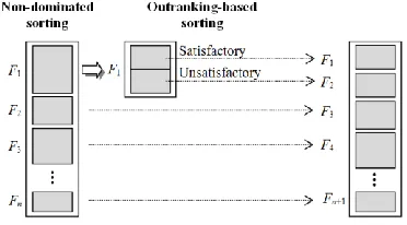
i. Calculate σ on F1×Tenh, where F1 is the non-dominated front of NSGA-II (the first front);
ii. Each solution x ∈ F1 is assigned by THESEUS to one category Ck of the set {satisfactory, unsatisfactory} by using Tenh as reference set;
iii. F1 is divided into two sub-fronts; the first ranked sub-front contains the solutions that were assigned to the most
preferred category (satisfactory);
iv. The remaining fronts of the current NSGA-II population are re-ordered by considering each sub-front of the original F1
as a new front; the NSGA-II’s elitism involves the new F1, which is now constituted by the non-dominated solutions
belonging to the most preferred category.
The above steps are illustrated in Fig. 3. In a MOP, the ROI should be composed of solutions that belong to the most preferred category. Hence, the solutions in the ROI are characterized by the fact that they are i) non-dominated, and ii) considered satisfactory solutions by the DM. Therefore, our approach creates a selective pressure towards solutions that have both features. In addition to incorporating the THESEUS method to search the ROI, our approach: a) uses diversity metrics according to the problem size; b) automatically enhances the reference set Tenh; and c) allows interaction with the DM to update his/her preferences. These processes are described in the following sections.
37
3.2.3 Diversity-preservation operators
As with any other genetic procedure, our method uses a diversity-preservation operator that is adapted according to the number of objective functions of the problem. In problems with three and four objectives, it is considered acceptable to use the well-known crowding distance based operator, where the density of solutions in the neighbourhood is measured [27]. However, as was stated in [42], the crowded-comparison operator is not suitable for many-objective optimization problems. For this reason, when dealing with many-objective problems (problems with five or more objectives), we use the reference point based operator of the recent proposal called Adaptive NSGA-III (A2-NSGA-III) [43], where the maintenance of diversity between population
members is aided by generating and adaptively updating a set of well-distributed reference points. This new operator incorporates the following operations: i) normalization of the values of the objective functions and the reference points in order to keep the ranges similar; ii) association of every population member with a specific reference point; iii) a niching procedure in order to ensure a diverse set of solutions; and iv) an update process that identifies those reference points that are not associated with a population member, allowing those points to be relocated by using addition and deletion strategies. These same actions are implemented in our method, with a slight adjustment in the normalization operation as recommended in [42].
3.2.4 An automatic procedure for enhancing the reference set
The reference set Tenh is automatically enhanced by the addition of some new solutions created during the search process. Each solution x F1, where F1 is the first sub-divided front (see Section 3.2.2 step iv), is considered in order to perform the automatic
enhancement of Tenh. A solution x belongs to the satisfactory category of Tenh if and only if the following two conditions are fulfilled:
i. x is assigned to the satisfactory category by THESEUS using Tupd as the reference set; ii. There is no solution b
Tenh such that b dominates x.These two conditions (called valid_assignation) are used in the enhancement process of Tenh that is described in Algorithm 2.
Algorithm 2. Automatic enhancement procedure
Input: F1, Tenh
Output: Tenh enriched
1. FOR each x F1 DO
2. IF x fulfils the conditions valid_assignation THEN
3. FOR each y satisfactory DO
4. IF x dominates y THEN
5. Remove y from satisfactory and incorporate it into
unsatisfactory
6. End FOR
7. Add x to satisfactory
8. ELSE
9. Add x to unsatisfactory
10. End FOR
11. Return Tenh enriched
12. End PROCEDURE
38
3.2.5 An interactive method for updating preferences
Our method takes advantage of the fact that the DM can progressively learn about the problem, thereby adjusting his/her preferences interactively, to drive the search towards the preferred zone of the Pareto optimal frontier (the ROI). For this, it is necessary to reflect the DM’s modified preferences by updating the current reference set. As was stated before, the DM’s preferences are reflected in Tupd, and therefore it is necessary to update this set. The updating is carried out as follows:
i. The satisfactory category of Tenh is presented to the DM who selects, from that set, the solutions that (s)he considers satisfactory according to his/her preferences.
ii. The solutions selected as satisfactory by the DM now form the new satisfactory category of Tupd. iii. The remaining solutions of Tenh now form the new unsatisfactory category of Tupd.
iv. After updating the DM’s preferences, do Tenh
Tupd.The updating of Tupd can be performed once in every certain number of iterations; this parameter is introduced as input at the beginning of the method. The number of updates depends on the time and effort that the DM is willing to spend. On the other hand, updating the DM’s preferences will help to eliminate possible inappropriate assignments suggested by THESEUS, since possible inconsistencies between the reference set and the preference model parameters can cause wrong assignments, as demonstrated in the study by Fernandez et al. [39]. Once the DM updates his/her preferences in Tupd, the same procedure as is described in Section 3.2.4 is applied to maintain the balance between the cardinality of the categories, if necessary.
4.
Some computer experiments
Let us consider two experiments that use the I-MCSGA to address the Public Project Portfolio Problem, which will be described in Section 4.3. In both experiments, we want to verify that our method leads to a good characterization of the ROI. We conduct the first experiment to determine whether the I-MCSGA is capable of obtaining better solutions than those obtained by the NSGA-II method in problems with three and four objectives; the second experiment explores whether our method outperforms A2-NSGA-III in many-objective problems (nine and sixteen objectives).
The configurations used in both experiments are outlined below.
In the first phase of the I-MCSGA, the NO-ACO algorithm (Section 2.2) is used to obtain an approximation to the Pareto frontier. This set of solutions is employed to construct the initial reference set Tupd. The NO-ACO parameters are the same as those reported in [32].
The parameters of the outranking model are set to the values suggested by Fernandez et al. in [2].
To ensure relatively fair conditions, the parameters for NSGA-II, A2-NSGA-III and the second phase of the I-MCSGA
are the same: crossover probability = 1; mutation probability = 0.01; the number of iterations = 500.
The data for the projects (e.g., cost, area, and region) are different for each instance.
The algorithms are programmed in the Java language, using the JDK 1.7 compiler, and NetBeans 7.1 as IDE, and they are run 30 times for each instance on a Mac Pro with an Intel Quad-Core 2.8 GHz processor and 3 GB of RAM.
In the absence of a real DM, we simulate him/her using the relational system of preferences proposed by Fernandez et al. [2] (Section 2.2). As a result, the creation of the initial reference set Tupd and its interactive updating is done by the preference model. These procedures are described below.
4.1 Constructing an initial reference set without a real DM
To construct the initial reference set Tupd, the solutions obtained by NO-ACO are categorized using the preference model. The categories considered to create the reference set are satisfactory and unsatisfactory. The reference set is constructed according to the following steps:
i. Run NO-ACO to find a set A of solutions containing a subset of the approximate Pareto frontier.
ii. Create the satisfactory category with those solutions belonging to the known Pareto frontier that satisfy |S(A, x)| = 0 (Eq. (6)), that is, that belong to the non-strictly-outranked frontier, and that also each of them fulfil one of the following conditions:
39
b. Is solution indifferent (Eq. (2)) to any solution in BS.c. Is a non-dominated solution (minimization) with respect to the objectives |W(A, x) | and |F(A, x) | in A. d. Has positive net flow score (Eq. (10)).
iii. Create the unsatisfactory category with the remaining solutions generated by NO-ACO in step i.
4.2 Updating the reference set without a real DM
To perform the updating of Tupd, the following steps are performed automatically:
i. Re-assign the solutions of the satisfactory category of Tenh using the simulated DM (Section 4.1 step ii).
ii. Create the new satisfactory category of Tupd with the solutions re-assigned by the simulated DM as satisfactory in Tenh. iii. Create the new unsatisfactory category of Tupd with the remaining solutions of Tenh.
iv. Apply the procedure described in Section 3.2.4 to maintain approximately the same number of reference elements in the two categories of Tupd.
v. Do Tenh
Tupd.4.3 Case study: A public project portfolio problem
Let us consider a decision-making situation in which the DM is in charge of selecting a group of projects (a portfolio) that will be implemented by his/her organization. The aim of this decision problem is to choose the ‘best’ portfolio that satisfies some budget constraints. Formalizing these concepts, let us consider a set of N projects, where the ith project is represented by a p-dimensional vector f(i) = ⟨f1(i), f2(i), f3(i), ... , fp(i)⟩, where each fj(i) indicates the contribution of project i to the jth objective. Each objective denotes the benefit target; that is, people belonging to a social category (e.g., Extreme Poverty, Poverty, Middle), who receive a benefit level (e.g., High Impact, Middle Impact, Low Impact) from the ith project.
On the other hand, a portfolio x is a subset of these projects, which is usually modelled as a binary vector x = ⟨x1, x2,..., xN⟩. In this vector, xi is a binary variable where xi = 1 if the ith project is supported and xi = 0 otherwise.
There is a total budget that the organization is willing to invest, which is denoted as B; each project has an associated cost ci. Portfolios are subject to the budget constraint:
1
.
Ni i i
x c
B
(15)The ith project corresponds to an area (e.g., health, education) denoted by ai. Each area has budgetary limits defined by the DM or another competent authority. Let us consider, for each area k, a lower and an upper limit, Lk and Uk respectively. Based on this, the constraint for each area k is
1
( )
.
N
k i i i k
i
L
x g k c
U
(16) where g is defined as
1
,
( )
.
0 otherwise
i i
if a
k
g k
(17) Besides, each project corresponds to a geographical region that will benefit from the project. In the same way as for the areas, each region has lower and upper limits as another constraint that must be fulfilled by a feasible portfolio.The quality of a portfolio x is determined by the union of the benefits of each of the projects that compose it. This can be expressed as
1 2 3
( )
( ),
( ),
( ),...,
p( ) .
z x
z x z x z x
z
x
(18) where zj(x), in its simplest form, is calculated as
1
( )
( ).
N
j i j
i
z x
x f i
40
If we denote by RF the region of feasible portfolios, the problem of the project portfolio is to identify one or more portfolios that solve
max{ ( )}.
F
x R
z x
(20) In this problem, the only accepted solutions are those portfolios that satisfy the following constraints: the total budget constraint (Eq. (15)), the area constraints (Eq. (16)), and the region constraints (similar to Eq. (16)).4.4 First experiment: NSGA-II vs I-MCSGA
[image:13.612.141.474.266.362.2]The first experiment consists of comparing the quality of the solutions provided by NSGA-II against those obtained from I-MCSGA in addressing problems with three and four objectives. We test six random instances whose basic information is shown in Table 4. In both algorithms, the population size is 100. The number of iterations to carry out the automatic enhancement is set to one. This means that the automatic enhancement process is performed at each iteration, namely 500 times. The number of iterations to execute the updating of the reference set Tupd is set to 200. That is to say, the updating is carried out only twice throughout the whole optimization process.
Table 4. Information about instances used in the first experiment.
Instance Instance Description
Objectives Projects
1 3 100
2 3 100
3 3 100
4 4 25
5 4 25
6 4 25
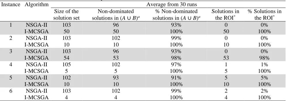
In Table 5, we present the average results of the 30 runs carried out for each instance. Instances 1–3 correspond to problems with three objectives. Although in this dimension NSGA-II is very competitive, the results reveal that on average our approach dominates between 1% and 7% of the solutions suggested by NSGA-II (Column 5). Conversely, in only one instance was there a solution of I-MCSGA that was dominated by a solution found by NSGA-II. No NSGA-II solution belongs to the satisfactory category, whereas almost all I-MCSGA solutions were satisfactory (Column 7). Instances 4–6 correspond to problems with four objectives. We can see that the solutions from our method dominate, on average, between 1% and 9% of the solutions suggested by II, whereas no I-MCSGA solution is dominated by any solution generated by II (Column 5). Besides, NSGA-II has very few solutions belonging to the satisfactory category, while all solutions of our method belong to the satisfactory category (Column 7).
Analysing the information contained in Table 5, we can observe that even though NSGA-II generates a larger number of solutions than I-MCSGA (Column 3), it fails to characterize the ROI, while our method always finds solutions belonging to the ROI.
Table 5. Comparative results between NSGA-II and I-MCSGA.
Instance Algorithm Average from 30 runs
Size of the solution set
Non-dominated solutions in (A ∪ B)a
% Non-dominated solutions in (A ∪ B)a
Solutions in the ROI*
% Solutions in the ROI*
1 NSGA-II 103 96 93% 0 0%
I-MCSGA 50 50 100% 50 100%
2 NSGA-II 103 102 99% 0 0%
I-MCSGA 10 10 100% 10 100%
3 NSGA-II 103 96 93% 0 0%
I-MCSGA 54 53 98% 53 98%
4 NSGA-II 105 102 97% 1 1%
I-MCSGA 5 5 100% 5 100%
5 NSGA-II 102 93 91% 5 5%
I-MCSGA 10 10 100% 10 100%
6 NSGA-II 103 102 99% 2 2%
I-MCSGA 4 4 100% 4 100%
[image:13.612.59.557.520.696.2]41
4.5 Second experiment: A2-NSGA-III vs I-MCSGA
The second experiment compares the quality of the solutions of A2-NSGA-III against those obtained from I-MCSGA, for
problems with nine and sixteen objectives. We test for four random instances, three of which are problems with nine objectives and the last of which is a problem with sixteen objectives. The basic information of these instances is shown in Table 6. The number of reference points in A2-NSGA-III is taken from the recommendations of Deb and Jain in [44]. The population size and
[image:14.612.139.473.184.253.2]number of reference points used in both algorithms are shown in Table 7. The parameters used for automatic enhancement and for updating the reference set Tupd are set as described in Section 4.4.
Table 6. Information about instances used in the second experiment.
Instance Instance Description
Objectives Projects
1 9 100
2 9 100
3 9 100
4 16 500
Table 7. Population size and number of reference points used by both algorithms. No. of objectives Population size No. of ref. points
9 174 174
16 136 136
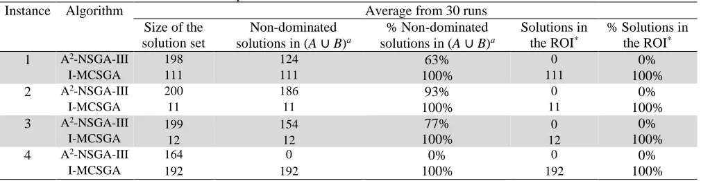
The comparative results are summarized in Table 8. Instances 1–3 correspond to problems with nine objectives. It can be seen that our method on average dominates between 7% and 37% of the solutions suggested by A2-NSGA-III, while the solutions
from I-MCSGA always remain as non-dominated (Column 5). There are no A2-NSGA-III solutions belonging to the satisfactory
category, while our method always finds non-dominated solutions belonging to the satisfactory category (Column 7). Instance 4 concerns a problem with sixteen objective functions. We can see that the solutions from our method dominate all of the solutions suggested by A2-NSGA-III, whereas no I-MCSGA solution is dominated by any solution generated by A2-NSGA-III
(Column 5). It is not surprising that no A2-NSGA-III solution belongs to the ROI, while our approach always finds satisfactory
[image:14.612.55.560.448.579.2]solutions (Column 7). These results give some evidence that our approach is effective in many-objective problems, providing a good characterization of the ROI.
Table 8. Comparative results between A2-NSGA-III and I-MCSGA.
Instance Algorithm Average from 30 runs
Size of the solution set
Non-dominated solutions in (A ∪ B)a
% Non-dominated solutions in (A ∪ B)a
Solutions in the ROI*
% Solutions in the ROI*
1 A2-NSGA-III 198 124 63% 0 0%
I-MCSGA 111 111 100% 111 100%
2 A2-NSGA-III 200 186 93% 0 0%
I-MCSGA 11 11 100% 11 100%
3 A2-NSGA-III
199 154 77% 0 0%
I-MCSGA 12 12 100% 12 100%
4 A2-NSGA-III 164 0 0% 0 0%
I-MCSGA 192 192 100% 192 100%
aA and B are the solution sets generated by A2-NSGA-III and I-MCSGA, respectively. *Solutions belonging to the approximated ROI (non-dominated and satisfactory)
5.
Conclusions and future work
42
The approach was verified through a method that we named I-MCSGA. We simulated the DM by using a preference model, with the parameters for the model remaining unchanged during the optimization process. The DM’s preferences are reflected by an outranking model and a reference set that is used by a multi-criteria sorting method (THESEUS) to assign new solutions to ordered categories. At a certain time, the solutions that were assigned as satisfactory by THESEUS during the search process are validated by a simulated DM to carry out the updating process of the preferences.
I-MCSGA was evaluated on project portfolio optimization problems, and we compared it with two methods from the literature. It was compared in relatively simple problems (three and four objectives) with NSGA-II and in many-objective problems (nine and sixteen objectives) with A2-NSGA-III. Our method showed better results than these methods with respect to
Pareto-dominance and also with respect to its capacity to reach the ROI.
The experimental results reveal that the elitism based on Pareto dominance combined with the category assignments performed by THESEUS help I-MCSGA to create selective pressure towards the ROI. The proposed automatic enhancement process is effective to incorporate new solutions into the reference set, helping THESEUS to suggest more appropriate assignments. Moreover, the suggested process of the interactive updating of preferences is effective in validating the solutions of the enhanced reference set, even when the real DM was replaced by a preference model. Therefore, the I-MCSGA, based on the proposed method, has shown its ability to characterize the ROI and to handle optimization problems with a few and many objectives efficiently.
Future research directions include extending the experimentation to problems where the true Pareto frontier is known, with the aim of validating the outcomes of our approach with greater certainty.
Acknowledgments
This work has been partially supported by PRODEP and the following projects: a) CONACYT Project 236154 and b) Project 269890 from CONACYT networks.
References
1. Coello, C.A., Lamont, G.B., Van Veldhuizen, D.A.: Evolutionary algorithms for solving multi-objective problems. 2nd edn, Springer, New York (2007).
2. Fernandez, E., Lopez, E., Lopez, F., Coello, C.A.: Increasing selective pressure towards the best compromise in evolutionary multiobjective optimization: The extended NOSGA method. Inform. Sciences, 181(1), pp. 44–56 (2011).
3. Machin, M., Nebro, A.J.: Multiobjective Adaptive Metaheuristics. Computación y Sistemas, 17(1), 53-62 (2013).
4. Lagunas, J.R., Moo, V.M., Ortíz, B.: Two-Degrees-of-Freedom Robust PID Controllers Tuning Via a Multiobjective Genetic Algorithm. Computación y Sistemas, 18(2), 259-273 (2014).
5. Deb, K.: Current trends in evolutionary multi-objective optimization. Int. J. Simul. Multi. Des. Optim. 1(1), pp. 1–8 (2007).
6. Miller, G.A.: The magical number seven, plus or minus two: some limits on our capacity for processing information. Psychol. Rev. 63(2), pp. 81–97 (1956).
7. Deb, K., Sundar, J., Udaya Bhaskara Rao, N., Chaudhuri, S.: Reference point based multi-objective optimization using evolutionary algorithms. International Journal of Computational Intelligence Research, 2(3), pp. 273–286 (2006).
8. Adra, S.F., Griffin, I., Fleming, P.J.: A comparative study of progressive preference articulation techniques for multiobjective optimisation. Evolutionary Multi-Criterion Optimization, Lecture Notes in Computer Science 4403, Springer-Verlag, pp. 908–921 (2007).
9. Bechikh, S.: Incorporating decision maker’s preference information in evolutionary multi-objective optimization. PhD thesis, University of Tunis, Tunisia (2013).
10. Sanchez, P.J.: Modelos para la combinación de preferencias en toma de decisiones: herramientas y aplicaciones. PhD thesis, University of Granada, Spain (2007).
11. Branke, J., Deb, K.: Integrating user preferences into evolutionary multi-objective optimization. Knowledge Incorporation in Evolutionary Computation, Studies in Fuzziness and Soft Computing, Springer-Verlag, pp. 461–477 (2005).
12. Zitzler, E., Brockhoff, D., Thiele, L.: The hypervolume indicator revisited: On the design of Pareto-compliant indicators via weighted integration. Evolutionary Multi-Criterion Optimization, Lecture Notes in Computer Science, Springer-Verlag, pp. 862–876 (2007). 13. Fowler, J.W., Gel, E.S., Köksalan, M.M., Korhonen, P., Marquis, J.L., Wallenius, J.: Interactive evolutionary multi-objective
optimization for quasi-concave preference functions. Eur. J. Oper. Res. 206(2), pp. 417–425 (2010).
14. Deb, K., Sinha, A., Korhonen, P.J., Wallenius, J.: An interactive evolutionary multiobjective optimization method based on progressively approximated value functions. IEEE T. Evol. Comput, 14(5), pp. 723–739 (2010).
43
16. Rachmawati, L., Srinivasan, D.: Incorporating the notion of relative importance of objectives in evolutionary multiobjective optimization. IEEE T. Evol. Comput. 14(4), pp. 530–546 (2010).
17. Bechikh, S., Ben, S.L., Ghédira, K.: The r-dominance: a new dominance relation for preference-based evolutionary multi-objective optimization. Technical Report BS-2010-001, SOIE Research Unit, High Institute of Management of Tunis, Tunisia (2010).
18. Deb, K., Kumar, A.: Interactive evolutionary multi-objective optimization and decision-making using reference direction method. In Proceedings of the 9th annual conference on genetic and evolutionary computation, ACM, USA, pp. 781–788 (2007).
19. Branke, J., Kaußler, T., Schmeck, H.: Guidance in evolutionary multi-objective optimization. Adv. Eng. Softw, 32(6), pp. 499–507 (2001).
20. Wagner, T., Trautmann, H.: Integration of preferences in hypervolume-based multiobjective evolutionary algorithms by means of desirability functions. IEEE T. Evol. Comput. 14(5), pp. 688–701 (2010).
21. Fernandez, E., Lopez, E., Bernal, S., Coello, C.A., Navarro, J.: Evolutionary multiobjective optimization using an outranking-based dominance generalization. Comput. Oper. Res. 37(2), pp. 390–395 (2010).
22. Oliveira, E., Antunes, C.H., Gomes, A.: A comparative study of different approaches using an outranking relation in a multi-objective evolutionary algorithm. Comput. Oper. Res. 40(6), pp. 1602–1615 (2013).
23. Köksalan, M., Mousseau, V., Özpeynirci, Ö., Özpeynirci, S.B.: A new outranking-based approach for assigning alternatives to ordered classes. Nav. Res. Log. 56(1), pp. 74–85 (2009).
24. Almeida-Dias, J., Figueira, J., Roy, B.: Electre Tri-C: a multiple criteria sorting method based on characteristic reference actions. Eur. J. Oper. Res. 204(3), pp. 565–580 (2010).
25. Hwang, C.L., Masud, A.S.M.: Multiple Objective Decision Making-Methods and Applications. Lecture Notes in Economics and Mathematical Systems 164, Springer-Verlag, (1979).
26. Deb, K., Kumar, A.: Light beam search based multi-objective optimization using evolutionary algorithms. IEEE Congress on evolutionary computation (CEC-07), Singapore, pp. 2125–2132, (2007).
27. Deb, K., Pratap, A., Agarwal, S., Meyarivan, T.: A fast and elitist multiobjective genetic algorithm: NSGA-II. IEEE T. Evol. Comput. 6(2), pp. 182–197 (2002).
28. Zitzler, E., Laumanns, M., Thiele, L.: SPEA2: Improving the strength Pareto evolutionary algorithm for multiobjective optimization. In Proc. Evolutionary methods for design, optimization and control with applications to industrial problems, pp. 95–100 (2002).
29. Ben Said, L., Bechikh, S., Ghédira, K.: The r-dominance: a new dominance relation for interactive evolutionary multicriteria decision making. IEEE T. Evolut. Comput. 14(5), pp. 801–818 (2010).
30. Pedro, L.R., Takahashi, R.H.: INSPM: An interactive evolutionary multi-objective algorithm with preference model. Inform. Sciences 268, pp. 202–219 (2014).
31. Miettinen, K., Ruiz, F., Wierzbicki, A.P.: Introduction to multiobjective optimization: interactive approaches. In Multiobjective Optimization, Lecture Notes in Computer Science 5252, Springer Berlin Heidelberg, pp. 27–57 (2008).
32. Cruz, L., Fernandez, E., Gomez, C., Rivera, G., Perez, F.: Many-objective portfolio optimization of interdependent projects with ‘a priori’ incorporation of decision-maker preferences. Appl. Math. Inf. Sci. 8(4), pp. 1517–1531 (2014).
33. Roy, B.: Multicriteria methodology for decision aiding, Nonconvex Optimization and Its Applications. Springer (1996).
34. Roy, B.: The Outranking Approach and the Foundations of ELECTRE methods. In Multiple Criteria Decision Aid. Bana e Costa CA (eds), Springer Berlin, pp. 155–183 (1990).
35. Brans, J.P., Mareschal, B.: PROMETHEE methods. In Multiple criteria decision analysis: state of the art surveys, Springer, pp. 163–190 (2005).
36. Fernandez, E., Navarro, J.: A new approach to multi-criteria sorting based on fuzzy outranking relations: The THESEUS method. Eur. J. Oper. Res. 213(2), pp. 405–413 (2011).
37. Doumpos, M., Zopounidis, C.: Multicriteria Decision Aid Classification Methods. Kluwer Academic Publishers (2002).
38. Fernandez, E., Navarro, J., Salomon, E.: Automatic Enhancement of the Reference Set for Multi-Criteria Sorting in The Frame of Theseus Method. Found. Comput. Decis. Sci., 39(2), pp. 57–77 (2014).
39. Fernandez, E., Navarro, J., Covantes, E., Rodriguez, J.: Analysis of the effectiveness of the THESEUS multi-criteria sorting method: Theoretical remarks and experimental evidence. TOP, pp. 1–26 (2016).
40. Fernandez, E., Navarro, J., Mazcorro, G.: Evolutionary multi-objective optimization for inferring outranking model’s parameters under scarce reference information and effects of reinforced preference. Found. Comput. Decis. Sci. 37(3), pp. 163–197 (2012).
41. Fernandez, E., Navarro, J., Duarte, A., Ibarra, G.: Core: A decision support system for regional competitiveness analysis based on multi-criteria sorting. Decis. Support Syst. 54(3), pp. 1417–1426 (2013).
42. Yuan, Y., Xu, H., Wang, B.: An improved NSGA-III procedure for evolutionary many-objective optimization. In Proc. of the 2014 conference on Genetic and evolutionary computation, USA, pp. 661–668 (2014).
43. Jain, H., Deb, K.: An improved adaptive approach for elitist nondominated sorting genetic algorithm for many-objective optimization. In Evolutionary Multi-Criterion Optimization, Springer Berlin Heidelberg, pp. 307–321 (2013).