A Study of the Elastodynamic Problem by Meshless Local Petrov Galerkin Method Using the Laplace Transform

(1)

http://www.scirp.org/journal/wjm ISSN Online: 2160-0503 ISSN Print: 2160-049X

DOI: 10.4236/wjm.2018.82004 Feb. 14, 2018 46 World Journal of Mechanics

A Study of the Elastodynamic Problem by

Meshless Local Petrov-Galerkin Method

Using the Laplace-Transform

Jaouad Eddaoudy, Touria Bouziane

Department of Physics, Faculty of Sciences, Moulay Ismail University, Meknes, Morocco

Abstract

The Meshless Local Petrov-Galerkin (MLPG) with Laplace transform is used for solving partial differential equation. Local weak form is developed using the weighted residual method locally from the dynamic partial differential equation and using the moving least square (MLS) method to construct shape function. This method is a more effective alternative than the finite element method for computer modelling and simulation of problems in engineering; however, the accuracy of the present method depends on a number of para-meters deriving from local weak form and different subdomains. In this pa-per, the meshless local Petrov-Galerkin (MLPG) formulation is proposed for forced vibration analysis. First, the results are presented for different values of

s

α _{, and} α_q_{with regular distribution of nodes} nt =55. After, the results are

presented with fixed values of αs and αq for different time-step.

Keywords

Meshless, MLPG, Weak Form, MLS, PDEs, Elastodynamic, Laplace Transform, Support Domain, Quadrature Domain, Regular Distribution

1. Introduction

Generality of physical or mechanical problems are modeled by partial differen-tial equations (PDEs). Moreover, a high number of numerical methods and techniques have been developed for the approximation of solution of the PDEs in much research that focused mainly on the improvement of accuracy and effi-ciency of them. In recent years, attention has turned on the development of meshless methods, especially for the numerical solution of partial differential

equations. The meshless local Petrov-Galerkin (MLPG) approach [1]-[14] has

How to cite this paper: Eddaoudy, J. and Bouziane, T. (2018) A Study of the Elasto-dynamic Problem by Meshless Local Pe-trov-Galerkin Method Using the Laplace- Transform. World Journal of Mechanics, 8, 46-58.

https://doi.org/10.4236/wjm.2018.82004 Received: December 19, 2017

Accepted: February 11, 2018 Published: February 14, 2018 Copyright © 2018 by authors and Scientific Research Publishing Inc. This work is licensed under the Creative Commons Attribution International License (CC BY 4.0).

http://creativecommons.org/licenses/by/4.0/

(2)

DOI: 10.4236/wjm.2018.82004 47 World Journal of Mechanics

become very attractive, as a promising method for solving problems. This me-thod based on a local weak form and Moving Least Squares (MLS)

approxima-tion [15][16][17][18]. The main advantage of this method over the widely used

ﬁnite element methods (FEM) is that it does not need any mesh, either for the interpolation of the solution variables or for the integration of the weak forms

[19][20]. The MLPG method and its variations have been applied for

elastody-namic and elastostatic problems by several authors. For example, it is applied to

free and forced vibration analysis for solids by Gu Y. T. et al. [21] they found

that the parameter which decides the size of the sub-domain needs to be chosen

carefully. Long S. Y. et al., have applied MLPG5 method used the Heaviside

function as the test function for elastic dynamic problems [22]. They found a

good agreement compared with the results obtained by (FEM). This method also

applied by Ping Xia et al. in elastic dynamic analysis of moderately thick plate

using meshless LRPIM [23]. They have used the Newmark method for solving

the dynamic problem and have studied the eﬀects of the size of the quadrature subdomain and the inﬂuence domain on the dynamic properties. They found if appropriate sizes are selected, good results and stability can be obtained. A meshfree-based local Galerkin method with condensation of degree of freedom

for elastic dynamic analysis by De-An Hu et al. [24], they have used the standard

implicit Newmark’s time integration scheme for solving the global dynamic sys-tem equations obtained by assembling all local discrete equations. Recent results

founded by Moussaoui and al concerning the effects of support domain αs for

elastostatic problem by MLPG [25].

The MLPG formulation is proposed in this paper to extend the MLPG method to dynamic analysis and for solving the problem of a thin elastodynamic

homo-geneous rectangular plate [26]. The Laplace transform [27] is applied to

elimi-nate the time variable, then, the obtained equations by the local formulation be-comes in function with coefficient of Laplace transform. The Stehfest inversion

method is applied to obtain the time-dependent solutions [28]. The result

pre-sented for different values of αs and αq with regular distribution of nodes

55 t

n = . After, the results are presented with fixed values of αs and αq for

different time-step. We found large domains of αs, αq and time-step by using

Laplace transform method. The integral equations have a very simple non-singular form. Moreover, both the contour and domain integrations can be easily carried out in rectangular sub-domains.

(3)

2. Moving Least Square (MLS) Approximation

We Consider a sub-domain Ωs the neighbourhood of point

( )

T ,

X = x y ,

which is located within the problem domain Ω_. _{To approximate a function}

(

X t,

)

u in Ωs, a finite set of monomial basis functions P

( )

X , is considered

in the space coordinates X in two-dimension is given by:

( )

[

]

T

1, ,

X = x y

P (1)

The approximation function of a field variable u

(

X t,

)

is defined in a

sub-domain Ωs by:

(

)

( ) (

)

T

( ) (

)

1

, m , ,

h

j j

j

X t =

∑

₌ p X a X t = X X t

u P a (2)

where P

( )

X is the monomial basis function of the spatial coordinates

( )

T ,

X = x y for two dimensional problem, and m is the number of the

mo-nomial basis functions. a

(

X t,

)

is a function of point X and time t and is a

vector of coefficients a X ti

(

,

)

given by:

(

X t,

)

=

{

a X t1

(

,

) (

a2 X t,

) (

a3 X t,

)

am

(

X t,

)

}

a (3)

The coefficient a

(

X t,

)

is obtained at any point X by minimizing a weigh-

ted discrete L2 norm

(

)

_T

( ) (

)

( )

2

1 ,

n

i i i

i= R X X  X X t u t 

=

∑

− _ − _

J P a (4)

where n is the number of nodes in the support domain of X for which the

weight function R X

(

−X_i

)

≠0, and u_i is the nodal parameter of u at

i

X =X .

The stationarity of J with respect to a

(

X t,

)

gives:

0

∂ ₌

∂ J

a (5)

which leads to the following linear relations:

( ) (

X X t,

)

=

( ) ( )

X t

A a B u (6)

where

( )

t

u is the vector that collects the nodal displacements for all nodes in the

support domain:

( )

{

( ) ( )

( )

}

T

1 2 n

t = u t u t u t

u (7)

( )

X

A is called the weighted moment matrix defined by:

( )

( ) ( ) ( )

T 1

n

i i i

i

X =

∑

₌ R X p X p X

A (8)

and the matrix B is defined by:

( )

X = R X p X1

( ) ( )

1 R2

( ) ( )

X p X2 Rn

( ) ( )

X p Xn 

B (9)

Solving a

(

X t,

)

from Equation (6) as:

(

)

1

( ) ( ) ( )

,

X t = − X X t

a A B u (10)

(4)

(

)

( ) ( )

T

( ) ( )

1

, n

h

i i

i

X t =

∑

₌ϕ X u t = X t

u Φ u (11)

where T

( )

X

Φ is the matrix of MLS shape functions corresponding n nodes in

the support domain of the point X and can be written as:

( )

{

( ) ( )

( )

}

_{( )}

( )

( ) ( )

T T 1

1 2 n ₁_n

X =

ϕ

X

ϕ

X

ϕ

X _× = p X A− X B X

Φ (12)

The shape function φi

( )

X for the i

th_{node is defined by:}

( )

(

1

( ) ( )

)

T

( )

(

1

)

1

m

i X j pj X A X B X ji X i

− −

=

∑

= p A B

φ ₍₁₃₎

The following quartic spline function is used, it has the following form of

( )

1 6 2 8 3 3 4 1

0 1

i i i i

i

r r r r

R r

r

 − + − ≤



=  _≥

 (14)

i i i X X r d − =

In which X−Xi is the distance from node Xi to point X, and di is

the size of the influence domain for the weight function.

3. Basic Equations of Elastodynamics

The governing equations for a linear two-dimensional elastodynamic problem on a domain Ω bounded by a boundary Γ are:

, in

ij j bi ui cui

σ + =ρ+ Ω (15)

(

, ,

)

in 2

i j j i ij

u u

ε = + Ω₍₁₆₎

in ijkl ij Dijkl

σ = ε Ω₍₁₇₎

where ρ_{the mass density,}_c_{is the damping coefficient,} 2₂i

i u u t ∂ = ∂

is the

acce-leration, i i u u t ∂ = ∂

the velocity, σij the stress tensor, bi the body force tensor,

and

( )

,j denotes

j

X

∂ ∂

The initial and boundary conditions are given as follows:

o

ˆ n

i i u

u =u Γ (18)

ˆ on

i ij j i t

t =σ n =t Γ (19)

(

)

( )

1 ,0 i0

u X t =u X X∈Ω (20)

(

)

( )

2 ,0 i0

u X t =v X X∈Ω (21)

where uˆ_i and tˆi are the prescribed displacement and traction on the

boun-dary Γu and Γt respectively, ui0 and vi0 denote the initial displacement

and initial velocity, nj is the unit outward normal to the boundary Γ. Γu

and Γt are complementary subsets of Γ.

(5)

( )

(

,

)

₀

( )

, e dst

( )

,

L f x t =

∫

+∞ f x t − τ= f x s (22)

( )

(

,

)

(

( )

,

)

( )

, 0

L f′ x t =sL f x s − f x (23)

( )

(

)

2

(

( )

)

( )

, , , 0 , 0

L f′′ x t =s L f x s −sf x − f′ x (24)

Then the Laplace-transform of the basic Equation (15) gives the general ex-pression of the partial differential equation:

(

)

(

)

2

(

)

(

)

, , , , ,

ij j X s scui X s s ui X s Fi X s

σ − −ρ = − ₍₂₅₎

where

(

,

)

(

, 0

)

(

, 0

)

(

, 0

)

(

,

)

i X s cui X sui X ui X b X si

F = +ρ +ρ + (26)

4. The MLPG Weak Formulation in Laplace-Transformed

Domain

The MLPG (meshless local Petrov-Galerkin) method constructs the weak form

over local subdomain such as Ωs, which is a small region taken for each node

inside the global domain. The local subdomains overlap, and cover the whole

global domain Ω_{. In the present paper, the local subdomains are taken to be of}

a quadrature shape. The local weak form [20][21] of the governing Equation (25)

can be written as:

(

)

(

2

)

(

)

( )

, , , ( , ) d 0, and 1, 2

s ij j i i i

X s sc s u X s F X s X i j

σ ρ

Ω  − + + Θ Ω = =

∫

(27)

where Θi

( )

X is a test function:

by using

(

)

, _, ,

ij j i ij i _j ij i j

σ

Θ =

σ

Θ − Θ

σ

₍₂₈₎

and applying the Gauss divergence theorem we can write:

(

) ( ) ( )

(

)

( )

(

)

(

) ( )

,

, d , d

d , , d

s s

ij j i ij i j

h

i s i i i

X s n X X X s

q X X s F X s X

σ σ

∂Ω Ω

Ω Ω

Θ Γ − Θ Ω

− Θ Ω = − Θ Ω

∫

u

∫

(29)

where

2

q=sc+ρs (30)

s

∂Ω _{is the boundary of the local subdomain, which is consisted of three parts,}

i.e.

s si st su

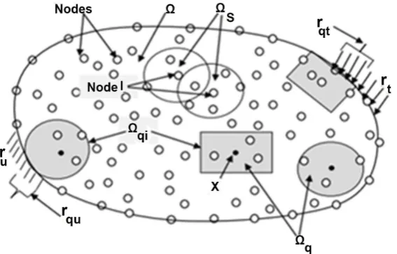
∂Ω = Γ ∪Γ ∪Γ (See Figure 1)

si

Γ _{is the local boundary that is totally inside the global domain,}

st

Γ _{is the part of the local boundary, which lies on the global boundary with}

prescribed tractions, i.e. Γ = ∂Ωst s∩Γt

su

Γ _{is the part of the local boundary that lies on the global boundary with}

prescribed displacements, i.e. Γ = ∂Ωsu s∩Γu

and considering:

(

,

)

(

,

) ( )

i ij j

(6)

[image:6.595.234.518.72.253.2]

Figure 1. The support domain ΩS and integration domain Ωq for node I.

The local weak form in Equation (29) is leading to the following local integral equation:

(

) ( )

(

) ( )

(

)

( )

(

)

(

) ( )

(

) ( )

,

, d , d , d

ˆ

d , , d , d

si su s

s st s

i i i i ij i j

L

h

i s i i i i i

t X s X t X s X X s

q X X s t X s X F X s X

θ θ σ

θ

Γ Ω

Ω Γ Ω

− Γ − Γ + Θ Ω

+ Θ Ω = Γ + Θ Ω

∫

u

∫

(32)

The strains can be obtained using the approximated displacements:

( )3 1

(

,

)

( ) ( )3 2 2 1

(

,

)

h

X s X s

× =L × u ×

ε ₍₃₃₎

Considering Equation (11) with Laplace transform:

(

)

( ) ( )

T

( ) ( )

1

, n

h

i i

i

X s =

∑

₌ϕ X u s = X s

u Φ u (34)

( )3 1

(

)

( )3 2 1

( ) ( )

( ) (3 2 2 2)

( )

(2 1)

( )

T

, ni i i n n

X s

ϕ

X u s X s

× =L ×

∑

= =L × Φ × u ×

ε

(35)

The constitutive equation gives the relationship between the stress and the strain:

(

,

)

(

,

)

ij X s =D ij X s

σ ε

(

,

)

1

( ) ( )

n

i i

i

X s =D

∑

₌B X u s

σ (36)

The traction vectors t X s_i

(

,

)

at a boundary point X∈∂Ω_s are

approx-imated by numbers of nodal values u si

( )

as:

(

,

)

(

,

) ( )

i ij j

t X s =σ X s n X

(

,

)

( )

1

( ) ( )

n

i i

i

X s = X

∑

₌ X s

t N D B u (37)

where the matrix N

( )

X related to the normal vector n_i of ∂Ωs by:

( )

1 2

2 1

0

n n

X

n n

 

=  

 

N (38)

(7)

( )

,1 ,2 ,2 ,1 0 0 i i i i i X ϕ ϕ ϕ ϕ     =      

B (39)

The stress-strain matrix D for plane stress is deﬁned by:

2 1 0 1 0 1 1 0 0 2

E _ν ν

ν _ν       = _ _ − _ _ −    

D (40)

In which E is the Young’s modulus and

ν

is the Poisson’s ratio.

Obeying the boundary conditions at those nodal points on the global boun-dary, where displacements are prescribed, and making use of the approximation formulae Equation (11), we obtains the discretized form of the displacement boundary conditions:

( ) ( )

(

)

1 ˆ , for

n

k k u

k=ϕ χ u s = χ s χ∈Γ

∑

u (41)

Substituting equations. (36) and (37) into Equation (32) we obtain the discre-tized Local integral equations:

( ) ( )

( )

( ) ( )

( )

( ) ( )

( )

(

) ( )

(

) ( )

d d

ˆ , d , d

si su

s s

st s

i i

i i s i s

i

X X X X X X

X q X X s

t X s X X s X

Γ Γ

Ω Ω

Γ Ω

− Γ − Γ





+ Ω + _{Ω }

= + Γ + Ω

∫

N DB N DB

W DB u

F Φ θ θ θ θ θ (42)

where θ

( )

X is a matrix of weight functions given by:

( )

_{( )}

0 0 i i X X X θ θ   =    

θ (43)

i

W is a matrix that collects the derivatives of the weight:

( )

, , , , 0 0 i x

i i y

i y i x

X X X X X θ θ θ θ     =      

W (44)

The cubic spline functions are used as the test functions for the local weak form:

( )

2 3

2

4 4 0.5

3

4 4

4 4 0.5 1

3 3 0 1 j i i i i i i i i

r r r

r r r r r

r θ  − + ≤   

= − + − < ≤



 >

 

(45)

where _i i .

i X X r d − =

(8)

size of the influence domain for the weight function.

Collecting the discretized local integral equations together with the discretized boundary conditions for displacements, we get the complete system of algebraic equations for computation of nodal displacements, which are the Laplace

trans-forms of ﬁctitious parameters uk

( )

p .

The time dependent values of the transformed variables can be obtained by an inverse Laplace transform. There are many inversion methods available for the

Laplace transformation. In the present analysis, the Stehfest algorithm [28] is

used. If g p

( )

is the Laplace-transform of g t

( )

, an approximate value g_a of

( )

k

g t for a speciﬁc time t is given by:

( )

1

ln 2 N ln 2

a i i

g t v g i

t = t

 

= _ _

 

∑

(46)

( )

_{( )}

(

) (

)

2 min , 2

2

1 2

2 ! 1

2 ! ! 1 ! ! 2 !

N i N

N i i

k i

k k

v

N k k k i k k i

+ = +_ _

= −

− − − −

∑

The selected number N = 10 with a single precision arithmetic is optimal to

receive accurate results. It means that for each time t, it is needed to solve N

boundary value problems for the corresponding Laplace parameters force

ln 2

s=i t with i=1, 2,,N. If M denotes the number of the time instants in

which we are interested to know g(t), the number of the Laplace transform

solu-tions g s

( )

j is then M × N.

5. Numerical Results and Discussions

In this section, numerical results will be presented to illustrate the implementa-tion and effectiveness of the proposed method. We present a numerical study for

elastodynamic 2-D problem of a rectangular homogeneous isotropic plate [26]

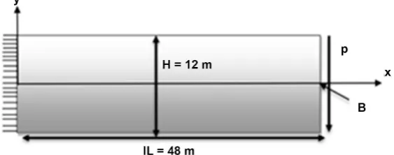
by using MLPG method, subjected to a dynamic force at the right end (Figure 2).

A plane stress problem is considered, and a unit thickness is used. The

dimen-sions of plate are length L=48 m and height H=12 m. The external

excita-tion force P=1.0f t

( )

, where f t

( )

=sin

( )

wt (simple harmonic load with

27 rad s

w= ) is a function of time, the damping coefficient c=0.4 is fixed for

all numerical computation. A total number nt =55 uniformly distributed

nodes is used, as shown in Figure 3, to represent the problem domain.

The dimension of the quadrature domain rq is set to dq=αqdc, where αq

is the size of the quadrature domain, dc is a distance to the ﬁrst nearest

neigh-bouring point from node i. The dimension of the inﬂuence domain ds is set to

s s c

d =α d , where αs is the size of the support domain.

The isotropic rectangular plate analyzed with the following material

proper-ties:

(

3

)

200 GP; 0.29; 7860 kg m

E= ν = ρ= in Steel. Some important

parame-ters on the performance of the method have been investigated.

Figure 4 displays the variations of displacements uy as a function of time at

point B under the harmonic load for different values of size of support domain

1.5,1.8,1.9, 2.0, 2.5 and 3.0 s

(9)

[image:9.595.232.514.76.187.2]

Figure 2. Rectangular homogeneous isotropic plate subjected to a

dynam-ic force at the right end of the plate.

[image:9.595.234.511.353.533.2]

Fgure 3. Conﬁguration and nodal arrangement for the plate.

Figure 4. Displacements uy at the middle point B at the free end of the

plate excited by the time-step load for different values of αs where 0.01 s

t

∆ = and α =q 2.0.

from this figure that the size of support domain inﬂuences on the results if

1.8 s

α < _{, and has a small effect on the results if} α >s 1.8). When α =s 3.0, the

results obtained by the present method is very good compared with the other

authors [21] that have used the Newmark method. In the following analysis,

3.0 s

α = is employed.

The time variation of displacements uy are given in Figure 5 with different

values of size of the quadrature domain αq, where ∆ =t 0.01 s. It is found that

the size of the quadrature domain αq inﬂuences seriously the results if

0.8 q

(10)

[image:10.595.226.521.74.263.2]

Figure 5. The time variation of displacements uy for different values of αq

where ∆ =t 0.01 s and α =S 3.0.

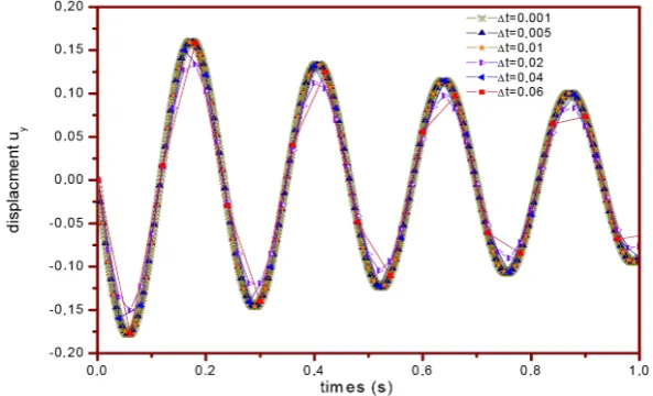
Figure 6. The time variation of displacements in the y direction at the point B

with different time steps ∆t using the fixed values αs=3.0,αq=2.0.

However, if the size of the quadrature domain is too large, the result obtained

for displacements by MLPG is great. We found good results with α_q=2.0

comparing with the results obtained by Long S. Y et al. [22], they have used

0.59 q

α = _.

Many time steps are used in computation to check the stability of the pre-sented MLPG formulation. The displacement variations as a function of time

and results for diﬀerent time steps are plotted in Figure 6. It can be found that

when the time step ∆t is less than 0.02 s, perfect results have been obtained

using the Laplace transform comparing with the results obtained by other

au-thors [23][24] that have used the Newmark method. It also can be found that

when a time step ∆t is larger than 0.02 s, the results are not convergent and not

[image:10.595.224.521.315.495.2]

(11)

6. Conclusion

The present method MLPG that uses the cubic spline test function is used to analyze elastodynamic problem. The equation formulation based on MLPG me-thod in Laplace transform and time domain with MLS approximation has been successfully implemented to solve elastodynamic problems in isotropic solids, subjected to a dynamic force at the right end of the plate. We found that the am-plitude of the vibration decreases with time because the effects of damping and the harmonic load, the response should converge to the static deformation. We

found that when the time step ∆t is less than 0.02 s, perfect results have been

obtained by using the Laplace transform and when a time step ∆t is larger than

0.02 s the results are not accurate. We found that the size of the quadrature

do-main αq has a small effect on the results if αq>0.8, and the size of the

sup-port domain αs influences on the results if α <s 1.8. The sizing parameters

s

α _and α_q_{, which decides the size of the subdomain needs to be chosen}

care-fully, especially, in the dynamic analysis.

References

[1] Atluri, S.N. and Zhu, T.L. (1998) A New Meshless Local Petrov-Galerkin (MLPG) Approach in Computational Mechanics. Computational Mechanics, 22, 117-127.

https://doi.org/10.1007/s004660050346

[2] Atluri, S.N. and Zhu, T.L. (2000) The Meshless Local Petrov-Galerkin (MLPG) Ap-proach for Solving Problems in Elasto-Statics. Computational Mechanics, 25, 169- 179. https://doi.org/10.1007/s004660050467

[3] Sladek, J., Sladek, V., Wen, P.H. and Aliabadi, M.H. (2006) Meshless Local Petrov- Galerkin (MLPG) Method for Shear Deformable Shells Analysis. CMES: Computer

Modeling in Engn. & Sciences, 13, 103-118.

[4] Sladek, J., Sladek, V., Zhang, C. and Solek, P. (2007) Application of the MLPG to Thermopiezoelectricity. CMES: Computer Modeling in Engn. & Sciences, 22, 217- 233.

[5] Mirzaei, D. and Dehghan, M. (2010) Meshless Local Petrov-Galerkin (MLPG) Ap-proximation to the Two Dimensional Sine-Gordon Equation. Journal of

Computa-tional and Applied Mathematics, 233, 2737-2754.

https://doi.org/10.1016/j.cam.2009.11.022

[6] Sladek, J., Stanak, P., Han, Z.D., Sladek, V. and Atluri, S.N. (2013) Applications of the MLPG Method in Engineering & Sciences: A Review. CMES, Computer Model-ing in Engn. & Sciences, 92, 423-475.

[7] Zhang, T., Dong, L.T., Alotaibi, A. and Satya, A.N. (2013) Application of the MLPG Mixed Collocation Method for Solving Inverse Problems of Linear Isotropic/Aniso- tropic Elasticity with Simply/Multiply-Connected Domains. CMES, Computer Mo- deling in Engn. & Sciences, 94, 1-28.

[8] Stanak, P., Sladek, V., Sladek, J., Krahuleca, S. and Sator, L. (2013) Application of Patch Test in Meshless Analysis of Continuously Non-Homogeneous Piezoelectric Circular Plate. Applied and Computational Mechanics, 7, 65-76.

(12)

DOI: 10.4236/wjm.2018.82004 57 World Journal of Mechanics [10] Sladek, J., Sladek, V. and Keer, R.V. (2003) Meshless Local Boundary Integral Equa-tion Method for 2D Elastodynamic Problems. International Journal for Numerical

Methods in Engineering, 57, 235-249. https://doi.org/10.1002/nme.675

[11] Qian, L.-F. and Ching, H.-K. (2004) Static and Dynamic Analysis of 2-d Function-ally Graded Elasticity by using Meshless Local Petrov Galerkin Method. Journal of

the Chinese Institute of Engineers, 27, 491-503.

https://doi.org/10.1080/02533839.2004.9670899

[12] Han, Z.D. and Atluri, S.N. (2004) Meshless Local Petrov-Galerkin (MLPG) Ap-proaches for Solving 3D Problems in Elasto-Statics. Computer Modeling in Engi-neering & Sciences, 6, 168-188.

[13] Han, Z.D. and Atluri, S.N. (2004) A Meshless Local Petrov-Galerkin (MLPG) Ap-proach for 3-Dimensional Elastodynamics. Computers Materials & Continua, 1, 129-140.

[14] Atluri, S.N., Han, Z.D. and Shen, S. (2003) Meshless Local Petrov-Galerkin (MLPG) Approaches for Solving the Weakly-Singular Traction & Displacement Boundary Integral Equations, CMES, 4, 507-517.

[15] Lancaster, P. and Salkauskas, K. (1981) Surfaces Generated by Moving Least Squares Methods. Mathematics of Computation 37, 141-158.

https://doi.org/10.1090/S0025-5718-1981-0616367-1

[16] Li, D., Wei, A., Luo, K. and Fan, J. (2015) An Improved Moving-Least-Squares Re-construction for Immersed Boundary Method, International Journal for Numerical

Methods in Engineering, 104, 789-804.https://doi.org/10.1002/nme.4949

[17] Shivanian, E. (2016) Local Integration of Population Dynamics via Moving Least Squares Approximation, Engineering with Computers, 32, 331-342.

https://doi.org/10.1007/s00366-015-0424-z

[18] Belytschko, T., Krongauz, Y., Organ, D., Fleming, M. and Krysl, P. (1996) Meshless Methods: An Overview and Recent Developments. Computer Methods in Applied

Mechanics and Engineering, 139, 3-47.

https://doi.org/10.1016/S0045-7825(96)01078-X

[19] Pandey, S.S., Kasundra, P.K. and Daxini, S.D. (2013) Introduction of Meshfree Me-thods and Implementation of Element Free Galerkin (EFG) Method to Beam Prob-lem. International Journal on Theoretical and Applied Research in Mechanical

En-gineering, 2, 2319-3182.

[20] Atluri, S.N., Cho, J.Y. and Kim, H.G. (1999) Analysis of Thin Beams using the Meshless Local Petrov-Galerkin Method with Generalized Moving Least Squares Interpolations. Computational Mechanics, 24, 334-347.

https://doi.org/10.1007/s004660050456

[21] Gu, Y.T. and Liu, G.R. (2001) A Meshless Local Petrov-Galerkin (MLPG) Method for Free and Forced Vibration Analyses for Solids. Computational Mechanics,27, 188-198.https://doi.org/10.1007/s004660100237

[22] Long, S.Y., Liu, K.Y. and Hu, D.A. (2006) A New Meshless Method Based on MLPG for Elastic Dynamic Problems. Engineering Analysis with Boundary Elements, 30, 43-48.https://doi.org/10.1016/j.enganabound.2005.09.001

[23] Xia, P., Long, S. and Cui, H. (2009) Elastic Dynamic Analysis of Moderately Thick Plate using Meshless LRPIM. Acta Mechanica Solida Sinica,22, 116-124.

https://doi.org/10.1016/S0894-9166(09)60096-3

(13)

DOI: 10.4236/wjm.2018.82004 58 World Journal of Mechanics [25] Moussaoui, A. and Bouziane, T. (2013) Comparative Study of the Effect of the Pa-rameters of Sizing Data on Results by the Meshless Methods (MLPG). World

Jour-nal of Mechanics, 3, 82-87.https://doi.org/10.4236/wjm.2013.31006

[26] Timoshenk, S. (1959) Theory of Plates and Shells. McGraw-Hill, New York, 2. [27] Davies, B. and Martin, B. (1979) Numerical Inversion of the Laplace Transform: A

Survey and Comparison of Methods. Journal of Computational Physics, 33, 1-32. https://doi.org/10.1016/0021-9991(79)90025-1

[28] Stehfest (1970) Algorithm 368: Numerical Inversion of Laplace Transform.