A Comparison of Machine Learning Classifiers
Applied to Financial Datasets
*
Abstract—The main purpose of this project is to analyze several Machine Learning techniques individually and compare the efficiency and classification accuracy of those techniques. Three algorithms are used (Naïve Bayes learning, feed forward Artificial Neural Networks with Backpropagation, and Decision Trees learning using C4.5) over two datasets (“European companies” and “Japanese companies”) characterized by 59 financial features each.
Index Terms—Financial datasets, Machine Learning algorithms
I. INTRODUCTION
Different kinds of machine learning algorithms are used today to help in activities where otherwise intensive human assistance is needed. Since the Machine Learning (ML) - statistics gap has experienced an outstanding reduction in the last years, ML methods have been applied for classification purposes as an alternative to purely statistical methods. This is due to the high accuracy ML methods show for certain analysis. There are many studies that compare different ML methods to find the most suitable for certain kinds of data. The research reported in [4] explained how ML methods can be used for traffic classification. This work showed that different ML algorithms (Bayes Net, Naïve Bayes Trees and C4.5) have similar performance in terms of classification. Also, in the area of financial information analysis some ML techniques have shown better results than statistical methods. For example, Artificial Neural Networks with Backpropagation performed better than discriminant analysis to predict bankruptcy in [10]. In another study [9], ML methods showed higher accuracy to predict home mortgage loan risk than the statistical method of probit analysis. This study also demonstrated how Decision Trees classifier outperformed other ML methods. Financial information classification is challenging because in general data under study is noisy, not stable and not Gaussian [8]. Since the analysis discussed in the present paper evaluates datasets of financial information, different ML techniques are considered to find the one that best classifies real stock information.
The purpose of the present research is to explore variance in European and Japanese markets’ stocks and examine the
* Manuscript received Jul 9, 2010. P. Robles-Granda. and I. Belik are with the
Computer Science Department, Southern Illinois University Carbondale, Carbondale IL USA 62901 Tel: 618-453-6630
Email: {pdrobles, ivanbelik}@siu.edu. Both authors contributed equally to this work.
performance of three types of ML algorithms to predict stocks volatility. This kind of study is of particular importance in financial analysis, for example in valuation. The rest of this paper is organized as follows: section II introduces methods, theoretical foundation, related works and experiments; section III presents the results; section IV describes the discussion, and finally section V presents the conclusions of the present work.
II. METHODS
A. ML algorithms description
Three types of algorithms were used to have a better perspective in the domain of the present analysis: Naïve Bayes learning, Artificial Neural Networks (Backpropagation) and Decision Trees learning. These three algorithms were chosen because of their different natures. Naïve Bayes learning is based on a probabilistic approach using Bayes' theorem. In spite of the fact that Naïve Bayes learning has a very simple mathematical basis, it can be used effectively for solving rather complicated problems. An example of the use of Naïve Bayes learning was described in [5]. This research showed the effectiveness of the Naïve Bayes classifier for the purpose of e-mail filtering and spam prevention.
Another approach uses Artificial Neural Networks, which is a kind of “Black Box” algorithm that usually uses a nonparametric approach and its performance does not depend on a priori or a posteriori knowledge about the area of interest. [2] Artificial Neural Networks are widely used in different spheres of life due to its useful features and capabilities like nonlinearity, input-output mapping, adaptivity, high fault tolerance, uniformity of analysis, and design. [6] One of the successful practical use of the Neural Network learning is the ALVINN system, which allows for the control of an autonomous vehicle using the principle of Backpropagation. [7]
Decision Trees learning is based on a “White Box” model and uses a predictive analysis. Decision Trees learning has been successfully used in many practical applications such as MARVIN [11], BACON [12], and INDUCE [13]. These systems became classical examples of the successful use of Decision Trees for classification tasks. Decision Trees learning is widely used because of its high-level of robustness, good performance with large data in a short time, and simple visualization and interpretation.
All of the ML techniques described above were used many
times in different areas, but research is still needed about their application in financial data processing. The nature of financial datasets is not completely formalized and certain because of social factors, which have a big influence in financial analysis. For this reason, the research represented in this paper shows how the ML algorithms can be applied to the classification of financial datasets and which level of efficiency the algorithms can provide.
B. Datasets description
Two datasets are used for the classification purposes. Each dataset represents the individual financial information for European and Japanese companies as of January, 2010. The “European Companies” dataset includes the characteristics of 4788 companies, and the “Japanese Companies” dataset includes 3644 companies [14].
These datasets are considered because they provide a big range of characteristic properties. They are used for hidden or indirect recognition of relations between features. The efficiency of this recognition is one of the basic characteristics of the analyzed algorithms. In fact, each algorithm should be able to provide an efficient relations’ recognition for correct classification.
The datasets were used to classify stock risk in terms of the remaining features. The volatility in the market is measured with the non-parametric value of variance in a stock: (High price - Low Price)/ (High price + low price). The higher this number, the more volatile the stock.
The financial characteristics belonging to both datasets have different levels of correlation between each other. For example, “Reinvestment Rate” and “EBIT (1-t)” are related directly [14]:
t) -(1 EBIT / in WC) Change + es Expenditur Capital
(Net
= Rate nt Reinvestme
(1)
Meanwhile, EBIT is directly related to EBITDA (EBITDA “estimated by adding depreciation and amortization back to operating income (EBIT)” [14]). Thus, there is indirect dependency between “Reinvestment Rate” and EBITDA. The efficiency of ML algorithms directly depends on their possibility to recognize all relations between training examples without antecedent knowledge about all economic and financial dependencies and consequently maximize the number of correctly classified examples. Thus, the given data sets represent a good experimental field for testing the efficiency of used ML algorithms and analyzing the level of dependency between given financial properties.
III. RESULTS (EXPERIMENT DESCRIPTION)
The experiments were performed over the datasets Eurocompfirm.xls and Japancompfirm.xls from Aswath Damodaran datasets [14] and applied three different ML algorithms: Naïve Bayesian learning, Decision Trees classifier and Artificial Neural Networks, as mentioned before.
The C4.5 algorithm was used for Decision Trees
classification and Backpropagation for Artificial Neural Networks. WEKA classification algorithms available at [15] were used for the Neural Networks testing of all the dataset in addition to WEKA machine learning workbench traditional package that includes the implementation for the Naïve Bayes learning and the Decision Trees learning algorithms.
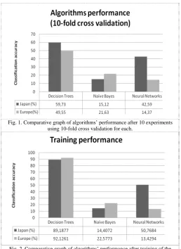
[image:2.595.298.557.233.588.2]Each algorithm was tested using 10-fold cross validation throughout 10 experiments for the “European companies” and “Japanese companies” datasets that tested around 4788 and 3644 entries respectively. Two phases of experiments are considered. The results for the two phases are shown in Fig. 1 and 2.
Fig. 1. Comparative graph of algorithms’ performance after 10 experiments using 10-fold cross validation for each.
Fig. 2. Comparative graph of algorithms’ performance after training of the original datasets.
A. Description of training performance
“Japanese companies” using the Naïve Bayes algorithm shows much lower efficiency (14.4%) compared to the Neural Networks implementation (50.7%). Nonetheless, both algorithms show a poor performance when compared with Decision Trees learning.
B. Description of classification performance.
As expected, the results after applying 10-fold cross-validation are worse than during the training. The efficiencies of all used algorithms were mostly decreased or not changed. As mention above, the Decision Trees algorithm gave the most significant performance during the training, and it also shows the most significant performance decrease after 10-fold cross validation. The efficiency decreased from 89.2% to 59.3% and from 92.1% to 49.5% for the “Japanese companies” and the “European companies” datasets respectively. The performance of the Naïve Bayes algorithm has been improved from 14.4% to 15.5% for the “Japanese companies” dataset, but it decreased from 22.6% to 21.7% using the “European companies” dataset. Largely, these insignificant deviations show good stability of the Naïve Bayes algorithm, even though the general performance is not high. Also, the performance of the Neural Network algorithm does not show any significantly positive changes. The efficiency of the Neural Networks algorithm using the “Japanese companies” has been decreased from 50.8% to 49.2%, and increased from 13.4% to 14.1% for the "European companies" dataset, but these differences are not significant for both cases. Thus, the most efficient result of classification is achieved using the Decision Trees algorithm for both datasets.
C. Analysis
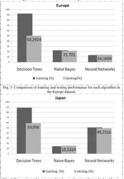
Fig. 3 and 4 depict algorithm training and testing performance comparison. As shown, Decision Trees learning shows the biggest difference of classification performance. The reason is that Decision Trees learning is a greedy approach that chooses the best solutions at hand when selecting classification features that are to be used for tests at each tree node. The solution is to prune the tree. However, in
[image:3.595.301.555.106.471.2]the experiments the learned trees were unpruned and this caused a big difference in classification performance.
Fig. 3. Comparison of training and testing performance for each algorithm in the Europe dataset.
Fig. 4. Comparison of training and testing performance for each algorithm in the Japan dataset.
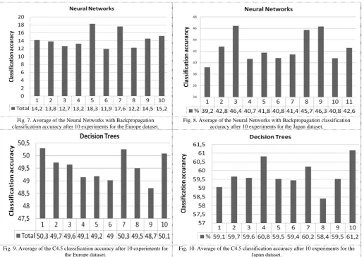
Fig. 5 – 10 depicts the classification accuracy of each respective algorithm per experiment. For each experiment 10-fold cross validation was performed. The figures were constructed by using the mean of each experiment.
[image:3.595.38.557.557.755.2]EUROPE JAPAN
Fig. 5. Average of the Naïve Bayes classification accuracy after 10 experiments for the Europe dataset.
Fig. 7. Average of the Neural Networks with Backpropagation classification accuracy after 10 experiments for the Europe dataset.
Fig. 8. Average of the Neural Networks with Backpropagation classification accuracy after 10 experiments for the Japan dataset.
Fig. 9. Average of the C4.5 classification accuracy after 10 experiments for the Europe dataset.
Fig. 10. Average of the C4.5 classification accuracy after 10 experiments for the Japan dataset.
It is important to notice that for the supervised learning (the Decision Trees algorithm) the “Risk Measure” feature was used as the key-feature (root test) for training and testing using WEKA. This feature was also used for the testing process for the Neural Networks and the Naïve Bayes algorithms. Originally, “Risk Measure” is a numeric feature with values in the range from 0 to 1. All “Risk Measure” values were classified into five groups giving symbolic names for each group. The classification process is described below.
IF “Risk Measure” < 0.2 THEN Risk_Class = "A"
ELSE
IF “Risk Measure” <0.4 THEN Risk_Class = "B"
ELSE
IF “Risk Measure” < 0.6 THEN Risk_Class = "C"
ELSE
IF “Risk Measure” < 0.8 THEN Risk_Class = "D"
ELSE Risk_Class = "E"
IV. DISCUSSION
Several experiments over two datasets and three different ML techniques were performed. As shown in the previous section, training and testing performance showed fairly different results. Isolated training results were in some cases better than the testing results because the classification obtained by training a ML algorithm can perform well with
the original training examples, but when testing the trained algorithm with different datasets, the performance is not always as predicted. For this reason, k-fold cross validation was used to have a more realistic measure of how the algorithms will perform in real case situations.
Using k-fold cross validation, performance differed from that shown in training; in some cases worsening it. It was particularly noticeable for the case of the Decision Trees learning, since the classification rate dropped to almost half of the original performance. Nonetheless, the Decision Trees learning was the technique that performed the best in terms of accuracy and also in terms of speed when compared to the Neural Networks algorithm. The Neural Network algorithm was the technique with the slower execution overall.
For a better analysis of results the comparison of 10-fold cross-validation and 2-fold cross-validation is done, and the results are represented in Table I.
Table I.The comparison of testing results using 10-fold/2-fold cross-validation
Algorithm
JAPAN EUROPE 10-fold
cross-validation (%)
2-fold cross-validation (%)
10-fold cross-validation (%)
The method of k-fold cross-validation shows the realistic outcome of the training process. The results given in Table I show the stability of all used ML techniques. Deviations between 10-fold cross-validation and 2-fold cross-validation results are not significant for all algorithms performed over both datasets. Predominantly, the deviation is not bigger than 1%. This situation means that some changes should be made to the parameters of the ML techniques for a better approach.
Some changes in parameters of the given algorithm should be realized to approach the best result of classification using Decision Trees learning:
1) Pruning: turn on the pruning procedure.
2) Changing of the confidence factor. Changing of the confidence factor makes the classification process more specific or more general depending on how close the training dataset is expected to be regarding the testing dataset. The value of the confidence factor should be decreased if the training and testing datasets are expected to be poorly related to each other. The decreasing of the confidence rate means that the tree will be more general. The default value of the confidence factor is 0.25.
3) Considering the subtree raising operator when pruning. It is the type of pruning that takes place when the node moves from zero-level of the tree up to the root, replacing other nodes along its way. It makes the computational process more complicated and does not guarantee a better approach.
Table II. The description of experiment results over datasets using Decision Trees learning
Experiment’s type Classification accuracy (%) “European companies” “Japanese companies” Original setting 49.55 59.73 “Pruning used” 49.85 60.027 “Confidence factor 0.1” 50.89 61.97 “Subtree raising operator
not used” 49.9 59.47
Originally, the Decision Trees algorithm was configured to run unpruned trees with a confidence factor of 0.25 in addition to the subtree raising operator usage. Table II above shows the result under this original setting and additionally it shows the result of changing each of these parameters independently. These values represent the average of 10 runs (experiments) of 10-fold cross-validation for each type of experiment.
As expected, by introducing pruning in the Decision Trees learning the classification accuracy value is increased for both datasets. Although this value is not significant in this case, the pruning process does increase the accuracy of classification. Similarly, the decrease in the confidence factor positively affects the accuracy performance of the algorithm for both datasets. Finally, whether subtree raising is included or not, the effect will not predict the utility of this option since for the case of the “European companies” dataset the accuracy increases while for the case of the “Japanese Companies” dataset the accuracy decreases. So it makes the computational process more complex, but it does not guarantee a better approach.
The decreased number of features, those which are the most discriminative, were taken for classification of the “European companies” dataset using the Decision Trees Learning based on 10-fold cross-validation. The purpose of this approach is to better classify the dataset. The results are represented in table III.
Table III. Classification results of the “European companies” dataset using the Decision Trees learning.
Number of
features % of correctly classified % of incorrectly classified 13 50.52 49.47
7 53.01 46.99
The experiments’ results given in table III show approximately the same outcome as for the 59-feature classification. It proves the stability of the Decision Trees learning and may show that the used datasets are noisy or the real dependencies between the analyzed financial features are weak.
V. CONCLUSION
During the project three different ML techniques were analyzed over two datasets. This analysis included detailed comparison of classification efficiency of used techniques. K-fold cross-validation was realized using each ML technique over each dataset.
The “Risk Measure”-feature is used for training and testing purposes in supervised learning (Decision Trees learning) and for testing purpose in the unsupervised techniques (Naïve Bayes learning and Artificial Neural Networks). The main interest is to analyze how the ML technique can learn to recognize the real economic relations and make the classification based on this information.
It was determined that the Decision Trees algorithm gives the best classification accuracy. Modification of its parameters was realized to get insights through a deeper analysis of this algorithm. The particular datasets under study were non Gaussian and noisy. The Decision Trees learning showed not only the best results but also the most homogeneous results throughout the entire experimental study.
Based on these initial results, obtained from the comparison of ML methods of the different natures, a deeper analysis of relations between real economic dependencies and the results of classification was performed using the seven and thirteen most discriminative features. In addition to the fact that stock behavior is rather stochastic, possible explanations for the results of this analysis are that the used datasets are noisy and that the real financial dependencies between the considered features are weak.
ACKNOWLEDGEMENTS
The authors would like to thank Dr. Norman Carver for his useful suggestions and comments about the experiments and Dr. Aswath Damodaran for the given datasets and help with financial concepts analyzed in this paper.
REFERENCES
[1] A. Johannet, B. Vayssade, and D. Bertin “Neural Networks: From Black Box towards Transparent Box Application to Evapotranspiration Modeling knowledge.” - World Academy of Science, Engineering and Technology 30 2007
[2] S.B. Kotsiantis “Supervised Machine Learning: A Review of Classification Techniques”, Informatica 31(2007) 249-268, 2007 [3] Turing, Alan (1952), "Can Automatic Calculating Machines be Said to
Think?", Copeland, B. Jack, The Essential Turing: The ideas that gave birth to the computer age, Oxford: Oxford University Press, ISBN 0-19-825080-0
[4] Nigel Williams, Sebastian Zander, Grenville Armitage (October, 2006)
A Preliminary Performance Comparison of Five Machine Learning Algorithms for Practical IP Traffic Flow. ACM SIGCOMM Computer Communication Review Classification
[5] M. Sahami, S. Dumais, D. Heckerman, E. Horvitz (1998). "A Bayesian approach to filtering junk e-mail". AAAI'98 Workshop on Learning for Text Categorization.
[6] Haykin, S. (1998). Neural Networks: A Comprehensive Foundation, 2nd edition. Prentice Hall, ISBN:0132733501
[7] Mitchell, Tom (1997). Machine Learning. New York: McGraw-Hill. ISBN 0-07-042807-7.
[8] Campbell J, Lo A, MacKinlay A. 1997. The Econometrics of Financial Markets. Princeton University Press: Princeton, NJ.
[9] Galindo J, Tamayo P. 2000. Credit risk assessment using statistical and machine learning: basic methodology and risk modeling applications.
Computational Economics 15: 107–143.
[10] Olmeda I, Fernandez E. 1997. Hybrid classifiers for financial multicriteria decision making: the case of bankruptcy prediction. Computational Economics 10: 317–335. [11] Sammut, C.A. (1985). Concept development for expert system
knowledge bases. Australian Computer Journal 17.
[12] Langley, P., Bradshaw, G.L., & Simon, H.A. (1983). Rediscovering chemistry with the BACON system. In R.S. Michalski, J.G. Carbonell and T.M. Mitchell (Eds.), Machine learning: An artificial intelligence approach. Palo Alto: Tioga Publishing Company.
[13] Michalski, R.S (1980). Pattern recognition as rule-guided inductive inference. 1EEE Transactions on Pattern Analysis and Machine Intelligence 2.
[14] Damodaran, A (2010).The Data Page. Retrieved from
http://pages.stern.nyu.edu/~adamodar/New_Home_Page/ (May, 4 2010) [15] The WEKA Classification Algorithms. Retrieved from