Proceedings of the CoNLL 2018 Shared Task: Multilingual Parsing from Raw Text to Universal Dependencies, pages 171–179 Brussels, Belgium, October 31 – November 1, 2018. c2018 Association for Computational Linguistics
171
NLP-Cube: End-to-end raw text processing with neural networks
Tiberiu Boros
Adobe Systems Romania
Stefan Daniel Dumitrescu
RACAI Romania
Ruxandra Burtica
Adobe Systems Romania
Abstract
We introduce NLP-Cube: an end-to-end Natural Language Processing framework, evaluated in CoNLL’s “Multilingual Par-sing from Raw Text to Universal Depen-dencies 2018” Shared Task. It performs sentence splitting, tokenization, compo-und word expansion, lemmatization, ta-gging and parsing. Based entirely on re-current neural networks, written in Py-thon, this ready-to-use open source system is freely available on GitHub1. For each task we describe and discuss its specific network architecture, closing with an over-view on the results obtained in the compe-tition.
1 Introduction and Shared task description
NLP-Cube is a freely available Natural Language Processing (NLP) system that performs:sentence splitting, tokenization, lemmatization, tagging andparsing. The system takes raw-text as input and annotates it, generating a CoNLL-U2 format file. Written in Python, it is based entirely on re-current neural networks built in DyNET (Neubig et al.,2017). The paper focuses on each NLP task, its architecture, motivating our choice and compa-ring it to the current state-of-the-art3
1
https://github.com/adobe/NLP-Cube
2The CoNLL-U format is well described in the official
Universal Dependencies (UD) websiteand in (Nivre et al.,
2018) and is the standard format of the UD Corpus. 3
We must note that in the official runs our system was affected by a bug which had a negative impact on the quality of the lexicalized features (See section2.1for details). Due to the fact that were unable to retrain the models to meet the Shared Task’s deadline (at the time of submitting this article we are still retraining them), we are reposting all new results on the GitHub project page.
The “Multilingual Parsing from Raw Text to Universal Dependencies” 2018 Shared Task ( Ze-man et al.,2018) targets primarily learning to ge-nerate syntactic dependency trees and secondarily the end-to-end text preprocessing pipeline (from raw text segmentation up to parsing), all in a mul-tilingual setting. The task is open to anybody, and participants can choose whether to focus on par-sing or attacking the end-to-end problem. The task itself is not simple, having to handle typologica-lly different languages, some of them having little or even no training data. Based on the Universal Dependencies (UD) Corpus4 (Nivre et al., 2016,
2018), participants have to target 82 languages, with datasets annotated in the CoNLL-U format. Their systems, given raw text as input, have to cor-rectly: segment a text into sentences (marked as SS in the results table, or Sentence Splitting), seg-ment sentences into words (marked as Tok, from Tokenization), expand single tokens/words into compound words (marked as Word), and, for each word, predict its universal part-of-speech (UPOS), language-dependent part-of-speech (XPOS), mor-phological attributes (Morpho), and dependency link to another word and its label, evaluated as 5 different metrics named CLAS, BLEX, MLAS, UAS, and LAS. Each of these metrics is well des-cribed in the Shared Task; for brevity, in this paper we will focus mostly on UAS - Unlabeled Attach-ment Score measuring only the linking to the cor-rect word, and LAS - Labeled Attachment Score, measuring both linking to another word and cor-rectly predicting the link’s label. Section 4 pre-sents NLP-Cube’s results for all these metrics for all languages in the Shared Task.
The paper is organized as follows: in section2
we first discuss generics, then move to each par-ticular task. We further present some training
pects of our system in section3, followed by re-sults in section 4, closing with section6on con-clusions.
2 Processing pipeline
The end-to-end system is a standard processing pi-peline having the following components: a sen-tence splitter, tokenizer, compound word expan-der (specific to the UD format), lemmatizer, tagger and a parser.
2.1 Input features
Our system is able to work with both lexicali-zed (word embeddings and character embeddings) and delexicalized, morphological features (UPOS, XPOS and ATTRs). However, we observed that when using morphological features as input (for example using POS tags as input for parsing), the performance of the end-to-end system generally degrades. This is mainly because while training is done using gold-standard morphological featu-res (e.g. the parser is trained on gold POS tags), at runtime these features are predicted at an earlier step and then used as “gold” input (e.g. the par-ser would be given tagger-predicted POS tags as input). There are several ways in which this effect can be mitigated with varying degrees of success; in our approach we preferred to use only lexicali-zed features as input for all our modules, with the exception of the lemmatizer which is heavily de-pendent on morphological information.
In what follows, when we refer to lexicalized features, we mean a concatenation of the fol-lowing:
1. external word embeddings:
300-dimensional standard word embeddings using Facebook’s FastText ( Bojanow-ski et al., 2016) vectors5 projected to a 100-dimensional space using a linear trans-formation); to these we included a trainable
<UNK>token;
2. holistic word embeddings: these repre-sent all words in the trainset which have a frequency of at least 2. They are 100-dimensional trainable embeddings, also in-cluding a<UNK>token for unseen tokens in the testset;
3. character word embeddings:
100-dimensional word representation generated
5Available ongithub.com/facebookresearch/fastText
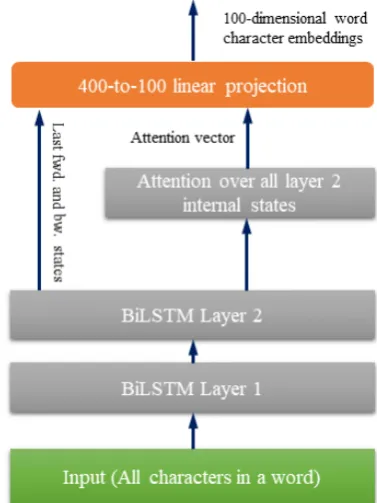
[image:2.595.322.511.115.367.2]by applying a network over the word’s symbols.
Figure 1: Word Character network for computing character-level features
The character word embeddings are obtained by applying a two-layer bidirectional LSTM network (size 200, using 0.33 dropout only on the recurrent connections) on a word’s characters/symbols (see Figure1). We then concatenate the final outputs from the second layer (top) forward and backward LSTM with an attention vector (totaling 400 va-lues: 100 from last fwd. state, 100 from last bw. state and 200 from the attention). The attention is computed over all the networkstates, using the final internal states of the top forward and bac-kward layers for conditioning. Letfk,(1,n) be the forward states of the top layer (k-th) in the cha-racter network andbk,(1,n)be its backward coun-terpart. Iffk,n is the forward state corresponding to the last character of a word andbk,1 is the bac-kward state of the first letter of that word, then the character-level embeddings (Ec) are computed as in Equations1,2and3.
si =V ·tanh(W1·(fk,i⊕bk,i)+
W2·(fk,n∗ ⊕b∗k,1)) (1)
αi =
exp(si)
Pn
k=1exp(sk)
Ec= n
X
i=1
αi·(fk,i∗ ⊕b∗k,i) (3)
Finally, we linearly project Ec to an 100-dimensional vector. Note, that we use f∗ andb∗
for theinternal statesof the LSTM cells and that the missing superscript means the variables refer to the output of the LSTM cells.
The morphological features are computed by adding three distinct (trainable) embeddings of size 100: one for UPOS, one for XPOS and one for ATTRS.
2.2 Tokenization and sentence splitting
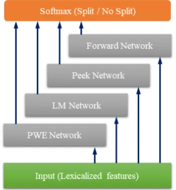
For most languages in the Shared Task our system uses raw text as input. Exceptions apply to the low-resourced languages for which we had little or no training data. In these cases we use the input provided by the UDPipe baseline system (Straka et al.,2016) which is already in CoNLL-U format. For tokenization and sentence splitting we use the same network architecture (see Figure2) and labeling strategy for all languages. The process is sequential: first we run sentence splitting and then we perform tokenization on the segmented senten-ces. In both steps, we use identical networks; ar-guably we could achieve both tasks in a single pass over the input data (the same architecture could perform both sentence splitting and tokenization). However, the best performing network parameters for sentence splitting are not identical to the best performing network parameters for tokenization. With this in mind, we trained two separate models for the two tasks.
For every symbol (si) in the input text, the de-cision for tokenization or sentence splitting (after
si) is generated using a softmax layer that takes as input 4 distinct vectors (final output states) of:
1. Forward Network: A unidirectional LSTM that sees the input symbol by symbol in natu-ral order;
2. Peek Network: A unidirectional LSTM , that peeks at a limited window of symbols6 in front of the current symbol - the input is fed to the network in reverse order;
3. Language Model (LM) Network: A
uni-directional LSTM that takes as input exter-nal word embeddings for previously
genera-6We set the value to 5 based on empirical observations
ted words; it updates only when a new word is predicted by the network;
4. Partial Word Embeddings (PWE)
[image:3.595.327.504.261.452.2]Ne-twork: It is often the case that we are able to generate valid (known) words made up of symbols from the previously tokenized word up to the current symbol. If the joined sym-bols form a word that exists in the embed-dings, we use these embeddings. Otherwise we use the unknown word embedding. We project the embedding using the same 300-to-100 linear transformation.
Figure 2: Tokenization and Sentence Splitting
For regularization, we observed that adding two auxiliary softmax layers (with same labels as final layer) for the Forward Network and the Peek Ne-twork slightly reduces overfitting. Intuitively, the Forward Network should be able to tokenize/sen-tence split based only on the previous characters and the Peek Network should also share this trait.
Moreover, the LM Network combined with the PWE Network should be able to “determine” if it makes sense (from the Language Modeling point-of-view) to generate another word, based on the previous words. This is highly important for lan-guages that don’t use spaces to delimit words in-side an utterance (e.g. Chinese, Japanese etc.).
2.3 Lemmatization and compound word expansion
Lemmatization (automatically inferring a word’s canonical form) and compound word expansion (automatically expanding collapsed tokens into their constituents) are similar in the sense that both start from a sequence of symbols and have the task of generating another sequence of symbols. One difference is that lemmatization is also depen-dent on the input word’s morphological attributes and part-of-speech, whereas compound word ex-pansion doesn’t have such data available (at least not for the UD corpus and consequently not for our system).
At first glance the two tasks can easily be sol-ved using sequence to sequence models. It is important to mention that by analyzing some in-put examples, one can easily see that inin-put-outin-put sequences have monotonic alignments. This im-plies that the standard encoder-decoder with atten-tion model is too complex and resource consuming for these two tasks.
We propose a method that uses an attention-free encoder-decoder model, which is less com-putationally expensive and, surprisingly, provides a 3-5% absolute increase in accuracy (at word le-vel) as opposed to its attention-based counterpart. The model is composed of a bidirectional LSTM encoder and an unidirectional LSTM de-coder. Similarly to a Finite State Transducer (FST) we train a model to output any symbol from the alphabet and three additional special symbols:
<COPY>, <INC> and <EOS>. During trai-ning, we use a dynamic algorithm to monotonica-lly align the input symbols to the output symbols. Based on these alignments, we create the “gold-standard” decoder output, which aims at copying as many input characters to the output as possible, while incrementing the input cursor and emitting new symbols only as a last resort.
Trying to find a comprehensive example for En-glish proves difficult (most lemmas are obtained by simply copying a portion of the input word) and we prefer to address lemmatization for a Ro-manian example because it allows a better explo-ration of the output sequence of symbols. A good example is the lemmatization process for the word “fetelor” (en.: girls), which has the canonical form “fat˘a” (en.: girl). The alignment process will ge-nerate the following source-destination pairs of in-dexes: 1-1, 3-3. The pairs map only symbols
that are identical in the input and output sequence. The output symbol list for the decoder to learn is:
<COPY>a<INC><INC><COPY>a<EOS>7. Let E(1,n) be the output of the encoder for a sequence ofninput symbols andibe an internal index which takes values from1ton. The algori-thm we use in the decoding process is:
E <− e n c o d e r ( word ) o u t <− ’ ’
i <− 1 do {
i n p = f ( E [ i ] , word ) c o u t = d e c o d e r ( i n p ) i f c o u t == ’<COPY>’
o u t <− o u t + word [ i ] e l s e i f c o u t == ’<INC>’
i <− i + 1
e l s e i f c o u t ! = ’<EOS>’ o u t <− o u t + c o u t } w h i l e ( c o u t ! = ’<EOS>’)
In the code above f(E[i], word) is generica-lly defined for both lemmatization and compound word expansion. The function uses the output of the encoder for positioniand, for lemmatization, it concatenates this vector with morphological fe-atures (see Section2.1for details). The compound word expander directly uses E[i] as input for the decoder.
To our knowledge, the attention-free encoder decoder provides state-of-the-art results8, our re-sults being up-to-par with the highest ranking sys-tem in the UD Shared Task. The results are repor-ted without using any lexicon for known words, and by employing the heuristic of leaving numbers and proper nouns unchanged.
2.4 Tagging
Tagging is achieved using a two-layer bidirectio-nal LSTM (same size for all languages). The in-put of the network is composed only of lexicali-zed features (see Section2.1) and the output con-tains three softmax layers that independently pre-dict UPOS, XPOS and ATTRS. Though the AT-TRS label is composed by multiple key-value pairs for each morphological attribute of the word (e.g.
7As a reviewer kindly noted, a <COPY> might not always be followed by an<INC>; We cannot exclude the possibility that a word in a certain language might have a sin-gle letter that has to be copied twice in the lemma. We thank the reviewer for pointing this out.
gender, case, number etc.), we treat the concatena-ted strings as a single value.
We performed a number of experiments trying to predict individual morphological attributes, but the overall accuracy degraded and we preferred this naive approach to other tagging strategies.
For regularization, we use an auxiliary layer of softmax functions (Szegedy et al.,2015), located after the first bidirectional LSTM layer. The ob-jective function is also designed to maximize the prediction probabilities for the same labels as the main softmax functions.
Note: The tagger is completely independent from the parser and we don’t use any morpholo-gical information for parsing.
2.5 Parsing
Our parser is inspired by Kiperwasser and Gold-berg(2016) and Dozat et al.(2017), in the sense that we use multiple stacked bidirectional LSTM layers and project 4 specialized representations for each word in a sentence, which are later aggrega-ted in a multilayer perceptron in order to produce arc and label probabilities.
We observed that training the parser on both morphological and lexical features biases the mo-del into relying on correct previously-predicted tags. This does not hold for end-to-end parsing, which implies that we use predicted (thus imper-fect) morphology. Also, in this Shared Task we can only train a tagger using the provided corpora, which means that it has access to the same features and training examples as the parser itself.
Taking all this into account, an interesting ques-tion arises: “Why would tagging followed by par-sing (learned on an identical training dataset) be better than multi-task learning and joint predic-tion of arcs, labels and POS tags?”. The answer that we came to is .. that it is not. Actually, we observed that jointly training a parser to also ou-tput morphological features increases the absolute UAS and LAS scores by up to 1.5% (at least for our own models).
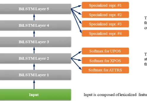
Our parser architecture (Figure 3) is composed of 5 layers of bidirectional LSTMs (sized 300, 300, 200, 200, 200). After the first two layers we introduce an auxiliary loss using three softmax yers for the three independent morphological la-bels: UPOS, XPOS and ATTRS. After the final stacked layer we project 4 specialized represen-tation which are used in a bi-affine attention for
predicting arcs between words and a softmax la-yer for predicting the label itself (after we decode the graph into a parsing tree).
There are several interesting observations which apply to this approach (but they could be generally true):
Observation 1: If we compute the accuracy of the auxiliary predicted tags and compare it to that of the independent tagger, we get an slight increa-sed accuracy for the UPOS labels and decreaincrea-sed figures for XPOS and ATTRS. This could mean that the contribution to parsing of the UPOS labels is higher than that of XPOS labels and morpholo-gical attributes. Of course, we are also using lexi-calized features, so this conclusion might be false. Note: In the end-to-end system we use the tagger to predict POS tags for UPOS, XPOS and ATTRS; the slight gain in accuracy of using UPOS tags pre-dicted by the parser are offset by the complexity of picking labels from separate modules and more parameter logic for the end-user of our system (for example, if a user requests only POS tags he wo-uld then need to run the parser just for UPOSes).
inte-Figure 3: Parser architecture
grated at training time and not just employed over an already trained network. However, the high computational complexity of this algorithm has a strong negative impact on the training time making it very hard to validate this theory.
3 Training details
Regarding drop-out, for all tasks we use a consis-tent strategy: similar to the methodology of Do-zat et al. (2017) we randomly drop each repre-sentation9 independently and we scale the others to cope with the missing input. The default para-meters used in our process are also close to those proposed in the aforementioned paper, with the ex-ception that we found a batch-size of 1000 to pro-vide better results. The batch size refers to the nu-mber of tokens included in one training iteration. Our models are implemented using DyNET ( Neu-big et al.,2017), which is a framework for neural networks with dynamic computation graph. This implies that we don’t require bucketing and pad-ding in our approach. Instead, when we compute a batch we add sentences until the total number of tokens reaches the batch threshold (1000). Often, we overflow the input size, because rarely the nu-mber of tokens sum up to exactly 1000.
The global early-stopping condition is that the task-specific metric over the development set do-esn’t improve over 20 consecutive training epochs. All models that use auxiliary softmax functions, weight the auxiliary loss by an empirically selec-ted value of 0.2. Whenever more than one aux
9For the tokenizer we even drop entire LSTM-outputs that represent the input of the final Softmax layer - but we still infer loss via the auxiliary softmaxes
softmax layers are used, the weighed value is equ-ally divided between the losses (i.e. if we use two auxiliary loss layers, each will infer a loss that is scaled with the value 0.1, not 0.2).
At runtime the end-to-end system performs the following operations sequentially: (a) it segments the input raw text using the best accuracy sentence splitter model, it then (b) tokenizes the sentences using the best accuracy tokenizer network model, (c) it generates compound words with the best ac-curacy compound word expander model over the tokens, (d) it predicts POS tags using each of the best performing network model for UPOS, XPOS and ATTRS respectively, (e) generates parse links and labels using the best UAS model (and not the LAS one, though we save this one as well), fina-lly (f) filling in the lemma with the best accuracy lemmatizer model.
We used the same hyperparameters for all lan-guages. They were chosen based on a few langu-ages that we initially tested on, and used these va-lues for all other languages. However, each task has its own set of hyperparameters that can be tuned individually. Except the input sizes (like the 300-to-100 linear transform in the tokenizer), all other LSTM sizes are configurable through the automatically generated config file for each task.
4 Results
[image:6.595.103.352.67.239.2]offi-177
Language Tok SS Word Lemma UPOS XPOS Morpho CLAS BLEX MLAS UAS LAS af afribooms 99.97 99.65 99.97 94.35 97.54 93.40 96.46 78.02 70.30 71.47 87.89 84.33 ar padt 99.98 77.35 91.10 48.65 87.71 84.37 84.58 64.96 33.12 58.13 71.53 67.61 bg btb 99.93 92.95 99.93 88.60 98.53 95.75 96.36 85.09 69.37 79.67 92.47 88.93 br keb 92.26 91.97 91.71 44.26 30.74 0.00 29.57 7.26 1.93 0.34 26.95 9.90 bxr bdt 83.26 31.52 83.26 16.05 34.99 83.26 37.95 1.01 0.03 0.06 6.32 2.42 ca ancora 99.98 99.27 99.94 97.49 98.45 98.51 97.94 86.24 83.57 82.54 92.91 90.49
cs cac 99.99 99.76 99.91 95.03 98.96 94.37 93.69 88.80 82.64 80.71 92.90 90.72 cs fictree 99.99 98.60 99.90 94.92 98.00 93.43 94.49 86.89 80.13 78.23 93.01 89.68 cs pdt 99.99 91.01 99.85 94.75 98.76 95.65 95.22 87.81 81.69 81.73 91.63 89.45 cs pud 99.55 91.70 99.40 92.22 97.17 92.93 92.04 81.96 75.30 72.76 89.60 84.82 cu proiel 100.00 37.28 100.00 80.96 93.23 93.52 85.27 65.68 54.38 53.66 74.60 67.70 da ddt 99.85 91.79 99.85 93.15 96.93 99.85 96.15 79.90 71.67 72.62 85.91 83.03 de gsd 99.70 81.19 99.62 76.71 93.83 96.78 88.54 72.96 42.49 54.79 82.09 77.24 el gdt 99.88 89.61 99.24 88.86 96.95 96.65 92.52 81.62 66.38 71.28 89.12 86.19 en ewt 99.26 76.32 99.26 94.51 95.25 94.83 96.03 79.31 73.77 73.75 85.49 82.79 en gum 99.65 82.13 99.65 91.70 94.71 94.42 95.64 75.01 65.38 67.42 84.10 80.59 en lines 99.91 87.80 99.91 93.89 96.38 95.01 96.46 75.40 67.82 69.28 82.58 78.03 en pud 99.74 95.70 99.74 94.32 95.14 93.88 94.99 82.36 76.12 72.76 88.27 85.31 es ancora 99.98 98.32 99.75 97.73 98.33 98.34 97.90 84.66 82.02 81.05 91.36 89.06 et edt 99.90 91.86 99.90 87.67 96.13 97.28 93.47 80.04 67.33 71.94 86.09 82.30 eu bdt 99.97 99.83 99.97 85.34 95.09 99.97 89.97 79.57 63.94 67.31 85.63 81.53 fa seraji 100.00 99.50 99.08 87.51 96.43 96.18 96.35 81.75 69.77 78.42 88.45 85.21 fi ftb 100.00 86.01 99.95 83.35 94.21 91.97 93.54 79.83 63.16 71.89 87.56 83.74 fi pud 99.67 93.29 99.67 76.66 96.59 0.03 94.56 85.14 58.90 78.41 90.05 87.28 fi tdt 99.70 88.73 99.70 77.92 95.52 96.52 92.41 81.74 58.42 73.04 87.06 83.74 fo oft 99.51 93.04 97.41 46.83 44.66 0.00 24.06 18.93 5.87 0.33 39.92 24.72 fr gsd 99.68 94.20 97.82 94.53 95.16 97.82 94.78 82.01 78.11 73.86 87.89 84.66 fr sequoia 99.86 89.86 97.77 93.35 96.08 97.77 95.19 81.91 76.06 75.50 87.83 85.27 fr spoken 100.00 21.63 100.00 90.62 95.22 97.45 100.00 57.63 52.78 53.41 72.76 65.81 fro srcmf 100.00 74.19 100.00 100.00 94.54 94.42 96.50 72.36 72.36 66.90 84.88 77.39 ga idt 99.56 95.38 99.56 84.98 91.01 90.40 79.78 53.98 41.89 35.54 76.80 65.37 gl ctg 99.84 96.59 99.17 94.93 96.86 96.30 99.04 75.10 69.73 68.20 83.90 81.07 gl treegal 99.50 84.99 95.06 84.67 90.25 86.75 88.27 57.80 46.62 47.68 71.13 64.90 got proiel 100.00 28.03 100.00 80.85 93.45 94.17 84.42 59.23 46.76 46.32 70.22 62.83 grc perseus 99.97 98.81 99.97 71.09 87.82 76.11 83.81 58.83 35.14 39.00 73.11 66.17 grc proiel 100.00 44.57 100.00 83.17 95.52 95.68 88.23 67.08 54.13 53.38 77.76 73.04 he htb 99.98 100.00 85.16 81.33 82.48 82.45 80.71 55.64 51.70 49.77 67.53 63.32 hi hdtb 99.98 98.84 99.98 96.71 97.16 96.49 93.25 87.30 84.70 76.01 94.65 91.27 hr set 99.92 95.56 99.92 89.95 97.72 99.92 90.52 82.77 71.56 69.81 90.64 85.81 hsb ufal 98.60 74.51 98.60 63.76 65.75 98.60 49.80 24.85 17.36 8.13 42.58 31.02 hu szeged 99.80 94.18 99.80 83.14 94.97 99.80 89.37 74.17 56.22 59.93 81.52 75.85 hy armtdp 97.21 92.41 96.47 70.79 65.40 96.47 57.07 23.40 17.36 10.44 44.53 29.63 id gsd 99.95 93.59 99.95 80.99 93.09 94.24 95.44 75.86 53.26 66.00 85.00 78.14 it isdt 99.75 96.81 99.68 96.88 97.79 97.63 97.54 85.53 81.42 81.57 92.49 90.21 it postwita 99.73 21.80 99.45 85.10 95.47 95.35 95.74 60.47 49.49 55.41 73.34 69.18 ja gsd 93.14 94.92 93.14 91.97 90.57 93.14 93.13 68.05 67.33 64.81 81.29 78.79 ja modern 65.98 0.00 65.98 54.14 47.71 0.00 64.15 4.42 4.07 2.76 16.67 13.60 kk ktb 92.26 75.57 92.89 23.49 57.84 56.04 38.32 13.15 0.76 2.69 39.48 19.64 kmr mg 94.33 69.14 94.01 64.64 59.31 58.77 48.39 17.91 11.69 5.87 34.86 24.18 ko gsd 99.87 93.90 99.87 38.39 95.27 88.24 99.70 79.75 21.93 76.44 86.10 82.09 ko kaist 100.00 100.00 100.00 30.05 95.12 84.14 100.00 83.63 15.26 79.50 88.13 86.00 la ittb 99.97 92.50 99.97 96.17 97.93 93.75 95.31 83.99 79.82 76.98 89.20 86.34 la perseus 100.00 98.67 100.00 67.55 85.69 68.29 72.63 45.39 28.48 29.01 63.46 51.92 la proiel 99.99 35.16 99.99 87.92 94.62 94.76 86.50 64.23 56.27 52.18 72.74 67.36 lv lvtb 99.68 98.05 99.68 86.24 93.73 83.09 88.44 74.87 61.18 61.31 83.41 78.18 nl alpino 99.89 90.75 99.89 92.76 95.68 93.80 96.07 80.42 71.95 72.73 89.32 85.95 nl lassysmall 99.84 77.48 99.84 92.47 95.83 94.12 95.45 75.26 66.41 69.25 85.37 81.75 no bokmaal 99.87 96.64 99.87 84.13 97.70 99.87 95.83 85.90 80.26 79.28 90.83 88.55 no nynorsk 99.96 94.28 99.96 82.42 97.42 99.96 95.41 85.90 76.43 78.33 90.83 88.53 no nynorsklia 99.99 99.86 99.99 75.80 85.36 99.99 81.19 48.26 40.44 35.31 64.43 52.94 pcm nsc 91.20 0.00 87.97 75.25 44.44 87.97 42.47 9.89 8.16 2.67 22.39 9.62
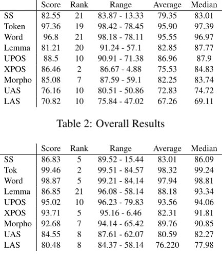
[image:7.595.127.478.71.773.2]Score Rank Range Average Median SS 82.55 21 83.87 - 13.33 79.35 83.01 Token 97.36 19 98.42 - 78.45 95.90 97.39 Word 96.8 21 98.18 - 78.11 95.55 96.97 Lemma 81.21 20 91.24 - 57.1 82.85 87.77 UPOS 88.5 10 90.91 - 71.38 86.96 87.9 XPOS 86.46 2 86.67 - 4.88 75.53 84.83 Morpho 85.08 7 87.59 - 59.1 82.25 83.74 UAS 76.16 10 80.51 - 50.86 72.83 74.72 LAS 70.82 10 75.84 - 47.02 67.26 69.11
Table 2: Overall Results
Score Rank Range Average Median SS 86.83 5 89.52 - 15.44 83.01 86.09 Tok 99.46 2 99.51 - 84.57 98.32 99.24 Word 98.87 5 99.21 - 84.14 97.94 98.81 Lemma 86.85 21 96.08 - 58.14 88.18 93.34 UPOS 95.02 10 96.23 - 79.83 93.56 94.06 XPOS 93.71 5 95.16 - 6.46 82.31 91.81 Morpho 92.68 7 94.14 - 65.42 89.76 90.85 UAS 84.55 8 87.61 - 62.07 80.59 82.27 LAS 80.48 8 84.37 - 58.14 76.220 77.98
Table 3: Results for Big Treebanks
cial website10 and due to space restrictions the description of each individual score is available online11 as well. For example, for sentence split-ting (SS) and tokenization (Token), the figures re-ported are F1 scores. For tables2and3we did not include in the max-min/average/median calcula-tion the lowest performing system as it had a very low score and would skew the overall ranking. For the Rank value in the tables please note that there were 25 systems participating (excluding the lowest competitor), so rank 10 means 10th posi-tion out of 25.
Overall, NLP-Cube performed above average for most tasks and treebanks, and, even better if we consider only the large treebanks. Due to the hidden bug we discovered very late in the TIRA testing period (mentioned in the introduction) we can see consistently bad performance for the tasks of compound word expansion and lemmatization where the character network has a large influence. Considering that for most languages we performed end-to-end processing, a low performance in the early processing chain compounded the error and led to lower scores.
5 Use-cases
We’ve built NLP-Cube with the vision that it wo-uld help in higher-level NLP tasks like Machine
10
http://universaldependencies.org/conll18/results.html
11http://universaldependencies.org/conll18/evaluation.html
Translation, Named Entity Recognition or Ques-tion Answering, to name a few.
Part of NLP-Cube, we have a Named Entity Recognition (NER) system12that employs Graph-Based-Decoding (GBD) over a hybrid network ar-chitecture composed of bidirectional LSTMs for word-level encoding, which had great results13.
We’re currently working on integrating Univer-sal Morphological Reinflection and also Machine Translation tasks in NLP-cube. We welcome fee-dback and contributions to the project, as well as new ideas and areas we could cover.
6 Conclusions
This paper introduces NLP-Cube: an end-to-end system that performs text segmentation, lemmati-zation, part-of-speech tagging and parsing. It al-lows training of any model given datasets in the CoNLL-U format. Written in Python, it is open-source, easily usable (“pip install nlpcube”) and provides models for the large treebanks in the Uni-versal Dependency Corpus.
We presented and discussed each NLP task. Results place NLP-Cube in the upper half of the best performing end-to-end text preprocessing systems. As we retrain our models, new scores will be continuously updated online14.
Finally, we highlight a few ideas:
1. We presented a lemmatizer / compound word expander that uses a Finite State Transducer-style algorithm that is faster and has better results than the classic attention-based encoder-decoder model (with the mention that it requires monotonic alig-nments between symbols) (see section2.3);
2. We obtained better results for Morphologi-cal Attributes when using each example as a sin-gle class instead of splitting and predicting their presence or not at every instance (see section2.4); 3. Parsing based on lexicalized features only, and at the same time, performing UPOS, XPOS and ATTRS prediction jointly with arc index and labeling led to a higher performance than parsing based on previously predicted morphological fea-tures generated by a tagger (see section2.5).
12
https://github.com/adobe/NLP-Cube/tree/dev.gbd-ner 13
http://opensource.adobe.com/NLP-Cube/blog/posts/1-gbd/results.html
References
Piotr Bojanowski, Edouard Grave, Armand Joulin, and Tomas Mikolov. 2016. Enriching word vec-tors with subword information. arXiv preprint ar-Xiv:1607.04606.
Timothy Dozat, Peng Qi, and Christopher D Manning. 2017. Stanford’s graph-based neural dependency parser at the conll 2017 shared task. Proceedings of the CoNLL 2017 Shared Task: Multilingual Parsing from Raw Text to Universal Dependenciespages 20– 30.
Eliyahu Kiperwasser and Yoav Goldberg. 2016. Sim-ple and accurate dependency parsing using bidirec-tional lstm feature representations. arXiv preprint arXiv:1603.04351.
Graham Neubig, Chris Dyer, Yoav Goldberg, Austin Matthews, Waleed Ammar, Antonios Anastasopou-los, Miguel Ballesteros, David Chiang, Daniel Clo-thiaux, Trevor Cohn, et al. 2017. Dynet: The dy-namic neural network toolkit. arXiv preprint ar-Xiv:1701.03980.
Joakim Nivre, Marie-Catherine de Marneffe, Filip Gin-ter, Yoav Goldberg, Jan Hajiˇc, Christopher Man-ning, Ryan McDonald, Slav Petrov, Sampo Pyysalo, Natalia Silveira, Reut Tsarfaty, and Daniel Zeman. 2016. Universal Dependencies v1: A multilingual treebank collection. InProceedings of the 10th In-ternational Conference on Language Resources and Evaluation (LREC 2016). European Language
Reso-urces Association, Portoroˇz, Slovenia, pages 1659– 1666.
Joakim Nivre et al. 2018. Universal Dependen-cies 2.2. LINDAT/CLARIN digital library at the Institute of Formal and Applied Lin-guistics, Charles University, Prague, http:
//hdl.handle.net/11234/1-1983xxx.
http://hdl.handle.net/11234/1-1983xxx.
Milan Straka, Jan Hajiˇc, and Jana Strakov´a. 2016. UD-Pipe: trainable pipeline for processing CoNLL-U files performing tokenization, morphological analy-sis, POS tagging and parsing. InProceedings of the 10th International Conference on Language Resour-ces and Evaluation (LREC 2016). European Langu-age Resources Association, Portoroˇz, Slovenia.
Christian Szegedy, Wei Liu, Yangqing Jia, Pierre Ser-manet, Scott Reed, Dragomir Anguelov, Dumitru Erhan, Vincent Vanhoucke, and Andrew Rabino-vich. 2015. Going deeper with convolutions. In
Proceedings of the IEEE conference on computer vi-sion and pattern recognition. pages 1–9.