http://www.scirp.org/journal/am ISSN Online: 2152-7393
ISSN Print: 2152-7385
DOI: 10.4236/am.2017.810107 Oct. 31, 2017 1464 Applied Mathematics
Investigation of the Class of the Rational
Difference Equations
Elmetwally M. Elabbasy
1, Osama Moaaz
1, Shaimaa Alsaeed
21Department of Mathematics, Faculty of Science, Mansoura University, Mansoura, Egypt 2Department of Mathematics, The Faculty of Education, Al al-Bayt University, Mafraq, Jordan
Abstract
This paper is concerned with asymptotic behavior of the solution of a new class of rational Difference Equations. We consider the local and global stabil-ity of the solution. Moreover we investigate the new periodic character (peri-odic two) of solutions of these equations. Finally, we give some interesting counter examples in order to verify our strong results.
Keywords
Difference Equation, Stability, Periodicity, Boundedness
1. Introduction
The objective of this work is to investigate the asymptotic behavior of the solu-tions of the following difference equation
0 1 1 3
1
1 2 1 3 2 4 3
, 0,1, 2,
n n
n
n n n n
b b
a n
c c c c
ω ω
ω
ω −ω ω −ω
+
− − −
= + + =
+ +
(1)
where a b b c c c, 0, , ,1 1 2, 3 and c4∈
[
0,∞)
and the initial conditions ω−3,,ω−1and ω0 are arbitrary positive real numbers.
In recent years, there are a great interest in studying the rational difference equations. These equations describe real life situations in queuing theory, sto-chastic time series, combinatorial analysis, electrical network, number theory, genetics in biology, psychology, probability theory, statistical problems, eco-nomics, etc. The study of rational difference equations of high order (greater than one) is a big challenge. However, there have not been any effective general methods to deal with the global behavior of rational difference equations of or-der greater than one. Therefore, the study of such equations is so interesting. There has been a lot of work concerning the global asymptotic of solutions of ra-How to cite this paper: Elabbasy, E.M.,
Moaaz, O. and Alsaeed, Sh. (2017) Investi-gation of the Class of the Rational Differ-ence Equations. Applied Mathematics, 8, 1464-1472.
https://doi.org/10.4236/am.2017.810107
Received: July 19, 2017 Accepted: October 28, 2017 Published: October 31, 2017
Copyright © 2017 by authors and Scientific Research Publishing Inc. This work is licensed under the Creative Commons Attribution International License (CC BY 4.0).
http://creativecommons.org/licenses/by/4.0/
DOI: 10.4236/am.2017.810107 1465 Applied Mathematics tional difference equations [1]-[21].
In fact, there has been a lot of interest in studying the behavior of the nonli-near difference equation of the form
1
1 .
n n
n
x x
x
α −
+ = +
(2) For multiple delay and order, see [3] [18] [19] [20] and their references for more results of this equation. In Theorems 4.7.1-4.7.5 in [12], Kulenovic inves-tigated the asymptotic behavior of the solutions of the equation
1 1
1
. n n
n n
x x
Bx Cx
γ −
+
− =
+ (3)
Metwally et al. in [14] established a global convergence result and then apply it to show that under appropriate hypotheses every positive solution of the dif-ference equation
1
0 2
, m
i n
i n i
A x
x +
= −
=
∑
where Ai∈
[
0,∞)
for i=0,1,,m. In [8], Elsayed studied the periodicity, theboundedness, and the global stability of the positive solution of the difference equation
1 1
1
,
n n
n
n n
x x
x
x x
α β γ −
+
−
= + +
where the parameters α β, and γ are positive real numbers and the initial
conditions x−1,x0 are positive real numbers. Recently, Moaaz et al. [15]
inves-tigated some qualitative behavior of the following nonlinear difference equations
1 ,
n l n l
n
n k n s
x x
x
x x
α β − γ −
+
− −
= + +
where the initial conditions x−r,x− +r1,,x0 such that r=max , ,
{
l k s}
arear-bitrary real numbers and α β, and γ are positive constants.
In this paper, in section 2, we state the sufficient condition for the asymptotic stability of Equation (1). Next, in section 3, we study the existence of periodic solutions of Equation (1). Finally, we study the boundedness nature of the solu-tions of Equation (1). Some numerical examples will be given to explicate our results.
During this study, we will need to many of the basic concepts. Before anything, the concept of equilibrium point is essential in the study of the dynamics of any physical system. A point ω in the domain of the function Φ is called an equilibrium point of the equation
(
)
1 , 1, , , 0,1, 2,
n n n n k n
ω
+ = Φω ω
− ω
− = (4) if ω is a fixed point of Φ [Φ
(
ω ω
, ,,ω
)
=ω
]. For a stability of equilibriumpoint, equilibrium point ω of Equation (4) is said to be locally stable if for all
0
DOI: 10.4236/am.2017.810107 1466 Applied Mathematics 0
k i i= ω− −ω δ<
∑
. As well, ω is said to be locally asymptotically stable if it is locally stable and there exists γ >0 such that, ifω
−ν∈(
0,∞)
for0,1, ,k
ν = with 0
k i i= ω− −ω γ<
∑
, then limn→∞ωn=ω. Also, ω is said tobe a global attractor if for every
ω
−ν∈(
0,∞)
for ν =0,1,,k , we have limn→∞ωn=ω. On the other hand, ω is said to be unstable if it is not locallystable.
Finally, Equation (4) is called permanent and bounded if there exists num-bers m and M with 0<m<M< ∞ such that for any initial conditions
(
0,)
νω
− ∈ ∞ for ν =0,1,,k there exists a positive integer N which depends on these initial conditions such that m<ωn<M for all n≥N.The linearized equation of Equation (1) about the equilibrium point
ω
ˆ is1 0 .
k
n i i n i
y+ =
∑
= p y−(5)
where
(
ˆ ˆ, , , ˆ)
. in i
F
p ω ω ω
ω− ∂ =
∂
Theorem 1.1 [12] Assume that pi∈ for i=0,1,,k. Then
0 1 k 1
p + p + + p <
(6) is a sufficient condition for the asymptotic stability of Equation(1).
2. The Stability of Solutions
The positive equilibrium point of Equation (1) is given by
0 1
1 2 3 4
ˆ a b b .
c c c c
ω = + +
+ +
Now, we define a function
(
(
) (
4)
)
0, , 0,
f∈C ∞ ∞ such that
(
)
0 11 2 3 4
, , , b v b r .
f u v w r a
c u c v c w c r
= + +
+ +
Therefore, we find
(
0 1)
21 2
, b c v f
u c u c v
∂ = −
∂ +
(7)
(
0 1)
21 2
, b c u f
v c u c v
∂ =
∂ +
(8)
(
1 3)
23 4
b c r f
w c w c r
∂ = −
∂ +
(9)
and
(
1 3)
23 4
. b c w f
r c w c r
∂ =
∂ +
(10)
Theorem 2.1. Assume that
ω
ˆ be a +ve equilibrium point of Equation (1).DOI: 10.4236/am.2017.810107 1467 Applied Mathematics
0 1 1 3 0 2 1 4 .
b cµ+b cλ<aλµ+b c µ+b cλ
where
(
)
21 2
c c
λ= + and
(
)
23 4
c c
µ= + , then
ω
ˆ is local stable. Proof. From (7) to (10), we get(
)
(
)
0 1 0 2 0 1 1 2 1 2 3 4ˆ ˆ ˆ ˆ, , , b c ,
f
p
u b b
a c c
c c c c
ω ω ω ω ∂ = − = ∂ + + + + +
(
)
(
)
0 1 1 2 0 1 1 2 1 2 3 4ˆ ˆ ˆ ˆ, , , b c ,
f
p
v b b
a c c
c c c c
ω ω ω ω ∂ = = ∂ + + + + +
(
)
(
)
1 3 2 2 0 1 1 2 1 2 3 4ˆ ˆ ˆ ˆ, , , b c
f
p
w b b
a c c
c c c c
ω ω ω ω
∂ = − = ∂ + + + + + and
(
)
(
)
1 3 3 2 0 1 1 2 1 2 3 4ˆ ˆ ˆ ˆ, , , b c .
f
p
r b b
a c c
c c c c
ω ω ω ω
∂ = =
∂
+ + +
+ +
Thus, the linearized equation of (1), is
1 0 1 1 2 2 3 3.
n n n n n
y+ =p y + p y− + p y− +p y−
From Theorem 1.1, we have that Equation (1) is locally stable if
(
)
(
)
(
)
(
)
0 1 0 1
2 2
0 1 0 1
1 2 1 2
1 2 3 4 1 2 3 4
1 3 1 3
2 2
0 1 0 1
1 2 1 2
1 2 3 4 1 2 3 4
1,
b c b c
b b b b
a c c a c c
c c c c c c c c
b c b c
b b b b
a c c a c c
c c c c c c c c
− +
+ + + + + +
+ + + +
+ − + <
+ + + + + +
+ + + +
and hence,
(
)
2(
)
2 0 1(
) (
2)
20 1 3 4 1 3 1 2 1 2 3 4 1 2 3 4
2b c c c 2b c c c a b b c c c c .
c c c c
+ + + < + + + +
+ +
Then, we find
(
)
(
)
(
)
(
)
(
)
(
)
2 2
0 1 3 4 1 3 1 2
2 2
2 2
1 2 3 4 0 2 3 4 1 4 1 2 ,
b c c c b c c c
a c c c c b c c c b c c c
+ + +
< + + + + + +
This completes the proof of Theorem 2.1.
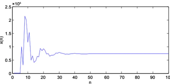
Example 2.1. Figure 1 shows that Equation (1) has local stable solutions if
0.01
a= , b0=200 , b1=20 , c1=0.002 , c2=0.01 , c3=0.002 and
4 0.001
c = .
DOI: 10.4236/am.2017.810107 1468 Applied Mathematics
Figure 1. The stable solution corresponding to difference Equation (1).
Equation (1) is global attractor.
Proof. We consider the following function
(
)
0 11 2 3 4
, ; , b v b r
f u v w r a
c u c v c w c r
= + +
+ +
(11)
Note that f non-decreasing for v r, and non-increasing for u w, . Let
(
ψ
,Ψ)
a solution of the system(
, , ,)
f
ψ
= Ψψ
Ψψ
(
, , ,)
f
ψ
ψ
Ψ = Ψ Ψ
From (11), we have
(
Ψ −a c)(
1ψ
+ Ψc2)
(
c3ψ
+ Ψ = Ψc4)
b0(
c3ψ
+ Ψ + Ψc4)
b1(
c1ψ
+ Ψc2)
and(
ψ
−a c)(
1Ψ +c2ψ
)
(
c3Ψ +c4ψ
)
=b0ψ
(
c3Ψ +c4ψ
)
+b1ψ
(
c1Ψ +c2ψ
)
Thus, we get(
a)(
)
b0(
)
b1(
)
,αβ
Ψ − Ψ +ψ
= Ψβ
Ψ +ψ
+ Ψα
Ψ +ψ
(12)
(
a)(
)
b0(
)
b1(
)
.αβ
Ψ − Ψ +ψ
=ψ β
Ψ +ψ
+ Ψα
Ψ +ψ
(13) By subtracting (12) and (13), we have
(
b0β
+b1α
)
(
Ψ −ψ
)
=0 Since b0β+b1α≠0, we get.
ψ Ψ =
This completes the proof of this Theorem.
3. Periodic Solution of Period Two
In this section, we investigate the existence of periodic solutions of Equation (1). Theorem 3.1. Assume that c1=c3=α and c2=c4=β. Equation (1) has
positive prime period-two solutions if
(
)(
)
(
2 2)
0 1 2 .
b +b α β− >a α +β + aαβ
DOI: 10.4236/am.2017.810107 1469 Applied Mathematics
Proof. Suppose that there exists a prime period-two solution
, , , , , , ,σ ρ σ ρ σ ρ
of Equation (1). We will prove that condition (14) holds. We see from Equation (1) that if c1=c3=α and c2=c4=β, then ωn=ωn−2=ρ, ωn+1=ωn−1=ωn−3=σ
and so,
0 1 0 1
1 2 3 4 1 2 3 4
and .
b b b b
a a
c c c c c c c c
σ σ ρ ρ
σ ρ
ρ σ ρ σ σ ρ σ ρ
= + + = + +
+ + + +
Thus, we have
2
0 1
a a b b
ασρ βσ
+ =αρ
+βσ
+σ
+σ
(15) and2
0 1 .
a a b b
ασρ βρ
+ =ασ
+βρ
+ρ
+ρ
(16) By subtracting (15) and (16), we have(
2 2)
(
)
(
)
(
)
(
)
0 1 ,
a a b b
β σ −ρ = − σ ρ− + β σ ρ− + σ ρ− + σ ρ−
then, we find
0 1.
a a b b
α β
σ ρ
β
− + + +
+ =
(17) By combining (15) and (16), we have
(
2 2)
(
)
(
)
(
)
(
)
0 1
2ασρ β σ+ +ρ =aα σ ρ+ +aβ σ ρ+ +b σ ρ+ +b σ ρ+
and so,
(
)
a(
a a b0 b1)
βσρ α β
− =α
−α
+β
+ +Since, 2 2
(
)
22
σ +ρ = σ ρ+ − σρ, we obtain
(
)
(
)
0 1aα aα aβ b b
σρ
β α β
− + + +
=
−
(18) Now,it is clear from (17) and (18) that σ and ρ are both two positive dis-tinct roots of the quadratic equation
(
)
2
0.
u + σ ρ+ u+σρ= (19)
Hence, we obtain
(
)
(
)
(
)
2
0 1 0 1
2
4
0,
a a b b a a a b b
α β α α β
β α β β
− + + + − + + +
− >
−
which is equivalent to
(
)(
)
(
2 2)
0 1 2 .
b +b α β− >a α +β + aαβ
This completes the proof of Theorem 3.1.
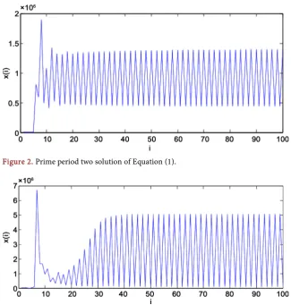
Example 3.1. Consider Equation (1) with c1=c4= =β 0.001,
3 4 0.002
c =c = =α , a=0.01, b0=200 and b1=20000. By Theorem 3.1,
Equation (1) has prime period two solution (see Figure 2).
DOI: 10.4236/am.2017.810107 1470 Applied Mathematics
Figure 2. Prime period two solution of Equation (1).
Figure 3. Prime period two corresponding to differences Equation (1).
0.005
α= , a=0.8, b0=500 and b1=2000. By Theorem 3.1, Equation (1)
has prime period two solution (see Figure 3).
4. Boundedness of the Solutions
In this section, we study the characteristic task of boundedness of the positive solutions of Equation (1).
Theorem 4.1. Every solution of (1) is bounded and persists. Proof. From Equation (1), we have
0 1 1 3 1
1 2 1 3 2 4 3
0 1 1 3
2 1 4 3
0 1
2 4
n n
n
n n n n
n n
n n
b b
a
c c c c
b b
a
c c
b b
a
c c
ω ω
ω
ω ω ω ω
ω ω
ω ω
− −
+
− − −
− −
− −
= + +
+ +
≤ + +
= + +
then,
0 1
2 4
0 n
b b
a M
c c
ω
< ≤ + + =
[image:7.595.213.535.72.233.2]DOI: 10.4236/am.2017.810107 1471 Applied Mathematics Conclusion 1. This work is concerned with studying a dynamics and behavior of solutions of a new class of difference Equation (1). Our results extend and ge-neralize to previous studies, for example, Equation (2)(if b1= =c1 0) and
Equa-tion (3)(if a= =b1 0). Furthermore, we obtain the following results:
- The +ve equilibrium point
ω
ˆ of equation (1) is local stable if0 1 1 3 0 2 1 4
b cµ+b cλ<aλµ+b c µ+b cλ , where λ=
(
c1+c2)
2 and(
)
2 3 4c c
µ= + .
Also, if c1=c2 and c3=c4, then
ω
ˆ is global attractor.- Equation (1) has a prime period-two solutions if c1=c3=α , c2=c4=β
and
(
)(
)
(
2 2)
0 1 2
b +b α β− >a α +β + aαβ.
- Every solution of (1) is bounded and persists.
Acknowledgements
The authors are grateful to the editors and anonymous referees for a very tho-rough reading of the manuscript and for pointing out several inaccuracies.
References
[1] Abdelrahman, M.A.E. and Moaaz, O. (2017) Investigation of the New Class of the Nonlinear Rational Difference Equations. Fundamental Research and Development International, 7, 59-72.
[2] Abdelrahman, M.A.E. and Moaaz, O. (2018) On the New Class of the Nonlinear Difference Equations. Electronic Journal of Mathematical Analysis and Applica-tions, 6, 117-125.
[3] Amleh, A.M., Grove, E.A., Georgiou, A. and Ladas, G. (1999) On the Recursive
Se-quence 1
1
n n
n
ω
ω α
ω−
+ = + . Journal of Mathematical Analysis and Applications, 233,
790-798.https://doi.org/10.1006/jmaa.1999.6346
[4] Camouzis, E., DeVault, R. and Ladas, G. (2001) On the Recursive Sequence
1 1 1
n n n
ω+ = − +ω− ω . Journal of Difference Equations and Applications, 7, 477-482.
[5] Elabbasy, E.M., EL-Metwally, H.A. and Elsayed, E.M. (2006) On the Difference Eq-uation ωn+1=aωn−bωn
(
cωn−dωn−1)
. Advances in Difference Equations, 2006, 1-10.[6] Elaydi, S.N. (1996) An Introduction to Difference Equations, Undergraduate Texts in Mathematics, Springer, New York.https://doi.org/10.1007/978-1-4757-9168-6
[7] Elsayed, E.M. and El-Metwally, H.A. (2012) Qualitative Studies of Scalars and Sys-tems of Difference Equations. Publisher LAP Lambert Academic.
[8] Elsayed, E.M. (2015) New Method to Obtain Periodic Solutions of Period Two and Three of a Rational Difference Equation. Nonlinear Dynamics, 79, 241-250.
https://doi.org/10.1007/s11071-014-1660-2
[9] Elsayed, E.M. (2016) Dynamics and Behavior of a Higher Order Rational Difference Equation. Journal of Nonlinear Sciences and Applications, 9, 1463-1474.
[10] Elsayed, E.M. (2010) On the Global Attractivity and the Periodic Character of a Re-cursive Sequence. Opuscula Mathematica, 30, 431-446.
https://doi.org/10.7494/OpMath.2010.30.4.431
DOI: 10.4236/am.2017.810107 1472 Applied Mathematics [12] Kulenovic, M.R.S. and Ladas, G. (2001) Dynamics of Second Order Rational Dif-ference Equations with Open Problems and Conjectures. Chapman & Hall/CRC.
https://doi.org/10.1201/9781420035384
[13] El-Metwally, H., Ladas, G., Grove, E.A. and Voulov, H.D. (2001) On the Global At-tractivity and the Periodic Character of Some Difference Equations. Journal of Dif-ference Equations and Applications, 7, 837-850.
https://doi.org/10.1080/10236190108808306
[14] Metwally, H.E., Grove, E.A. and Ladas, G. (2000) A Global Convergence Result with Applications to Periodic Solutions. Journal of Mathematical Analysis and Applica-tions, 245, 161-170.https://doi.org/10.1006/jmaa.2000.6747
[15] Moaaz, O. and Abdelrahman, M.A.E. (2016) Behaviour of the New Class of the Ra-tional Difference Equations. Journal of Mathematical Analysis and Applications, 4, 129-138.
[16] Moaaz, O. (2017) On Comment on “New Method to Obtain Periodic Solutions of Period Two and Three of a Rational Difference Equation. Nonlinear Dynamics, 79, 241-250.https://doi.org/10.1007/s11071-016-3293-0
[17] Moaaz, O. and Abdelrahman, M.A.E. (2017) On the Class of the Rational Difference Equations. International Journal of Advances in Mathematics, 4, 46-55.
[18] Ocalan, O. (2014) Dynamics of the Difference Equation ωn+1=pn+ωn k− ωn with a
Period-Two Coefficient. Applied Mathematics and Computation, 228, 31-37. [19] Saleh, M. and Aloqeili, M. (2005) On the Difference Equation xn+1= +A x xn n k− .
Applied Mathematics and Computation, 171, 862-869.
[20] Sun, T. and Xi, H. (2007) On Convergence of the Solutions of the Difference Equa-tion n 1 1 n 1
n ω ω
ω
−
+ = + . Journal of Mathematical Analysis and Applications, 325, 1491-1494.
[21] Zhang, L., Zhang, G. and Liu, H. (2005) Periodicity and Attractivity for a Rational Recursive Sequence. Journal of Applied Mathematics and Computing, 19, 191-201.
https://doi.org/10.1007/BF02935798