Stability Behavior of the Zero Solution for Nonlinear Damped Vectorial Second Order Differential Equation

(1)

Stability Behavior of the Zero Solution for Nonlinear

Damped Vectorial Second Order Differential Equation

Mohamed A. Ramadan1, Samah M. El-Kholy2

1_{Department of Mathematics, Faculty of Science, Minufiya University, Shebeen El-koom, Egypt}

2_{Department of Engineering Physics and Mathematics, Faculty of Engineering, Kafr El-Sheikh University, Kafr El-Sheikh, Egypt}

Email: [email protected], [email protected], samahelkholy77@ yahoo.com Received October 7, 2012; revised November 9, 2012; accepted November 18,2012

ABSTRACT

In this paper, a theoretical treatment of the stability behavior of the zero solution of nonlinear damped oscillator in the vectorial case is investigated. We study the sufficient conditions for the boundedness of solution of the nonlinear damped vectorial oscillator and the conditions for the stability of the zero solution to be uniformly stable as well as asymptotically stable.

Keywords: Zero Solution; Damped Oscillator; Uniformly Stable; Asymptotically Stable

1. Introduction

We consider the nonlinear second order vectorial differential equation of the form

 

2f t  t t,

  

x x x g x 0

.

R

(1) where;





 

   

1, , ,2

, : ,and , :

,

n

,

n

n n

t R x x x R

t R R R f t  t R



 

  

  



x

g x

Stability problems for the second order ordinary differential equation has been intensively and widely studied [1-5]. Based on Schauder fixed point theorem T. A. Bur- ton and T. Furumochi [2] introduced a new method to study the stability of the zero solution for Equation (1). This problem is considered also by Gheorghe Morosanu and Cristian Vladimirescu [5,6]. In [6], they used rela- tively classical arguments to prove the stability of the zero solution of Equation (1). While in [5], they obtained new stability results for this ordinary differential equation under more general assumptions. Their approach al- lows extensions to both the vector case and the case of the whole real line. In [7] the dynamics of various oscil- lators had been studied.

2. The Main Results

In the next theorem we state sufficient conations for the boundedness of the solution of Equation (1) are given.

Theorem 1

If the following hypotheses are hold: 1)

 

1

 

f t C R and f t

 

  0, t 0.

2)

 

1

 

_,

t C R

 _  _ _{is decreasing and}

 

₁

t

  ,

t R

  .

3)



n



R ,

n C R R

 

g and g is locally Lipschit- zian

in



x1, , xn



,

4) g satisfies the following estimate

 

t,  f t o

 

g x x ,  t R , where _ denotes

some norm in . then the solution of Equation (1) is bounded.

n R

Proof

For the n-dimensional system, we have





T

1, , , , , , ,2 1 2

m

n n

x x x y y y R

 _ _ 

z , where m = 2n.

Applying the transformation, yi  xi f t x

 

i and 1, 2, ,

i  n Equation (1) can be converted into a first order system of differential equations of the form:

 



,



A t B t t

   

z z z r z (2)

where

1)

 

1 2

3 4

A t A t

A t

A t A t

 

  

  and are

m × m matrices.

 

1

0 0

0

B t

 

  

 

2) A t1

 

A t4

 

 f t I

 

, A t2

 

I,

 

3

A t   t I , and B t₁

 





f2

 

t  f

 

t



I

0n n

are n × n matrices. Note that,  and I are the zero and the

identity matrices, respectively.

3) r

 

t,x 0  g t1

 

,x  gn

 

t,x T

 

1 0

,

n

t



 

 

 



g x

which is a 2m1 vector.

For i j, 1, 2, ,_ n, let is an arbitrary fixed

and let 0

0

(2)

 

11 0 12 0 1 0

, ,

21 0 22 0 2 0

0

, ,

1 0 0

, , ,

,

, ,

m

i j i n j m

n i j n i n j

mm m

z t t z t t z t t

Z Z

z t t z t t z t t

Z t t

Z Z

z t t z t t



  

 

 

 

 

 

 

 

 

 

 

 

(3)

be a fundamental matrix solution to the linear system:

 

A t

 

z z (4)

which equal to the identity matrix for ₀. Consider with

tt

00

z z₀ small enough, and

let us denote by

0 0

t 



t t, ,0 0



z z

0 z

the unique solution of Equa- tion (2) which equal to  at tt0. By hypotheses (1) and (2), z



t t, ,0 z0



is defined on a maximal right inter-

val,



t l₀,



, and satisfies the following integral equation:





 

    







0

1

0 0 0 0 0 0 0 0 0 0

, , , , , , , , , , d

t

t t Z t t 



Z t t Z s t _B s s t  s s t _ s

z z z z z r z z

This gives us the following integral inequality:





 

  







0

1

0 0 0 0 0 0 0 0 0 0

, , , , , e , , , , , d

t

t t  Z t t 



Z t t Z s t _B s s t  s s t _ s

z z z z z r z z (5)

where e



0 _ 1 0 _



T.

Equations (3) and (4) give us the following differential equations:

 

, ,

i j i j n i j

z  f t z z__,

,

 

,

(6)

 

, ,

n i j i j n i j

z_   t z  f t z_ (7)

 

, ,

i n j i n j n i n j

z _  f t z _ z (8)

 

, ,

n i n j i n j n i n j

z_ _   t z _ f t z _ _ (9)

for i j, 1, 2, ,_ n.

 



Since is a decreasing function, so Equations (6) and (7) lead to:

t

 

2 2

   

2 2

, , , ,

1

2  t zi j zn i j f t  t zi j zn i j 

      

  

 

0  

2 d

2 2

, , 0 e

t

t f u u

i j n i j

t z z t

  _    (10)

By the same way we can obtain from Equations (8) and (9) the following:

 

0  

2 d

2 2

, , e

t

t f u u

i n j n i n j

t z z

    



  (11)

For



1, , , , , , ,2 1 2



T

m

n n

x x x y y y R

 _ _ 

z , consider

the norm 2

1

m

i i

z 





z , where  is the norm defined

in m.

R

 For





T

0 01, 02, , 0 , 01, 02, , 0

m

n n

x x x y y y R

 _ _ 

z we

have:

 









, , 0 , 0 , 0

0 0

, , 0 , 0 , 0

2 2

, 0 , 0 , 0 , 0

1 1 1

, i j i n j i j i n j

n i j n i n j n i j n i n j

n n n

i j j i n j j n i j j n i n j j

i j j

Z Z Z Z

Z t t

Z Z Z Z

z x z y z x z y

 

     

   

  



    

 _ __{ }  _ _

  

   

_ _ _ 

 

 _  _ _ 

   

 

 



x y

x z

x y

y

  

satisfies (4), then we get: Using Shwartz inequality, Minkowski inequality [8] and

suitable assumptions lead to:

 

0  

2 d

0 0 0 0

, 3 1e

t

t f u u

Z t t n  t

 

 

z z (12)

We have also:

0 0

t s t

   

 













1

0 0

T

1 0 2 0 0

, , e

, , , , _m , ,

Z t t Z s t

t s t t s t t s t

  



 

   

 





 













1

0 0

0 1

2 2

0 0

1

, , e

, , , ,

i i

n

i i n

i

Z t t Z s t

t t s t t s t

  





 







Since

2 _{, ,}

m

t s t







 

t

 is a decreasing function of , we get:

(3)

  

2



2





  

2



2





0 0 0 0

, , , , , , , , e S

  2tf udu

 

i n i i n i

t t s t t s t s s s t s s t

      

    

   

So,

 

1

 

 d

0 0 0

, , e

t

S

f u u

Z t t Z s t e n t



 _  ₍₁₃₎

As mentioned the system satisfies the integral inequality (5), then inequalities (12) and (13) give





 

   

 









0

1

0 0 0 0 0 0 0 0 0 0

, , , t , , e , , , , , d

t

t t Z t t Z t t Z s t _B s s t s s t _ s

 

 





z z z z z r z z





 

0  

 

  



 

d d

2

0 0 0 0 0 0 0

, , 3 1e e

t t

t tS

f u u t f u u

t t n  t n t n f s

 

0

t

, , , d

f s s t s s

    

  



_ _

z z z

For all t we can replace g by another function say g

defined as follows. By hypothesis (4) it follows that there exists a

z z g x (14)

0

  such that if x , then

 

t, f t o

 

g x x

We defined the function : n n by:

RR R



g

 

, if

,

, if

g t t

g t

 

 

ave

  

 



x x

g x

x x

and we h x_ ,  t 0.

ry ,x

It is clear that for eve

 

t RRn

 

t, 

 

g x f t o x

is of class and is locally Lipschitzian 

g

in





n C RR



x x1, , ,2  xn



ginal function. So, we wg satisfies

 

ill admit from now that the all the properties of the

ori g.

Since 1

f C R we get from inequality (14) that:





 





0

0 0 0 0

, , 3 1e

t

t f u

t

t t n t

D

 

 





0

0 0

, , d

t

s t s

du

z z z

u g

z z



0,



t t l

  , with positive constant D [9,10]. This gives s the followin



t t, ,0 0



n 3

 

t0 1eDh 0 , t



t l0,



z z z (15)

Thus z



t t, ,₀ z₀



as well as z



t t, ,₀ z₀



are bounded

on



t l₀,



and so z



t t, ,₀ z₀



can be extended to the

right of l. This contradicts the maximality of l. This means that the solution of Equation (1) is bo nded. The proof of theorem 1 is complete.

Theorem 2

If the hypotheses of theorem 1 are hold and lowing assumption is satisfied:

1) There exist two constants such that: u

the fol-

, 0

h k

 

2

 



_,



f t  f t kf t  t h 

then the zero solution of Equation (1) is uniformly stable solution.

If in addition



2)

 

0

d

f t t 



holds, then the zero solution of Equation (1) is asymptotically stable.

Proof n

Our stability question is reduced to the stability of the zero solutio z

 

t 0

will be divided into two intervals. In the

to the system (2). The interval of

t first interval

we have t



t h0,



and in the second interval t



h,



. lh and si

on a ma

Firstly, with nce the hypotheses of theorem 1 are hold, and then the solution z



t,t z₀, ₀



of Equation

l right interval

(1) is defined xima



t l0,



. It is

proved in theorem 1 that the solution is bounded and



t t, ,0 0



z z can be extended to the right of l. Therefore,



t t, ,0 0



z z exists on



t l₀,



with lh.

Assume h  l . We are going to find an estimate for z



t t, ,0 z0



on the interval



h l,



. From hypothesis

(1) of theorem 2, we have for  t



h l,



:





 





 



 



, ,



 

,



d

t u

nk f s z s t z  g s x s

d d

0 0 0 0

, , 3 1e , e

t

S S

t

f u u f u

t t n  h h t n h

 

  

z z z ,z₀

h



0 0



0,



 

 d



,







 d









 





t

h S

f u u

n  h  nk f s f s

 

z₀ z₀ ₀ ₀

h

0 0 0 0

e , , , , d

t f u u

s t  s t s





z z x z

, 3 1e ,

t

t t  h t n h







(4)

with

 

1

0, nk

n h





 

 

 

 

 

(16)





 





 







 





0 0

d

0 0 0

d

0 0

, ,

3 1e , ,

e t

h

t

S

f u u

t f u u

h

t t

n h h t

n h nk f s s t s



 



 



 







z z

z , ,z d

(17)

 





 





 





d

0 0 0

d

0 0

3 1e , ,

e ,

t

h

t

S

f u u

t f u u

h

v t h h t

n h nk f s s t s



 



 



 







z z

So

, d

 

  



1

   



,



v t _ n h nk  _f t v t  t h l .

By integration we get:





 

    





1 d

0 0

, , e ,

,

t

h

n h nk f u u

t t t h

t h l

v v

 

  

 

 

 

z z ₍₁₈

with

)

 

3

 

1



, ,0 0



v h n  h  z h t z

From inequality (18) we can see that z



t t, ,0 z0



is

bounded since z



t t, ,₀ z₀



is also bounded, it foll s

that For

ow l .  0 we can get:

 







 



2

e

1 3 0 1 3

Dh

n h

   

 



 

From (15) it follows that





 

0 0

, ,

1 3

t t

n h

 

 

z z

for all t

 

t h0, provided that z0  ore,

from (16) and (18), we get z



t t, ,₀ z₀



v h. Theref

 

 for all th. So, if 0t₀h, then the solution





starting , ,0 0

t t

z z

from any point z₀, with z₀  , exists on



t0,



and satisfies z



t t, ,0 z0



 for al

usly we btain that l 0

tt . If

and:

0

t h, then analogo o l 





 

    



0

1 d

0 e ,

t

nh nk  f u u

  

 



(19



,

t h

 

Therefore, with the same

0 0 0

, , 3 1

t t n  t 

z z z ₎

t

 as before, z₀ 

im-plies again



t t, ,0 z0



 Hence the

If in

z for all tt₀.

zero solution is uniformly stable. addition

 



0

d

f t t 



is satisfied, then by (16), (18) and (19) it follows tha zero solution to (1) is asymptotically stable. The proof of

theorem 2 is complete.

3. Examples

We confirm the results of the introduced theorems by considering two numerical examples for which the func-tions

t the

 

f t , 

 

t and g

 

t satisfy theorems assump-

tions.

For the system

 



 

2f t  t,

  t



 0

x x x g x

where

,



x x1, 2



x .

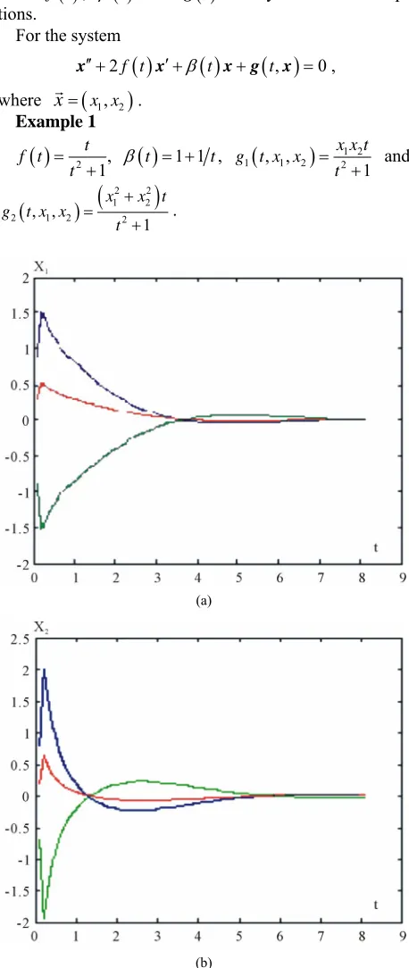
Example 1

 

2 ₁

t f t

t



 , 

 

t  1 1t,





1 2 1 , ,1 2 2 ₁

x x t g t x x

t



 and







12 22



2 , ,1 2 2 ₁

x x t

g t x x

t

 

 .

(a)

[image:4.595.309.538.165.707.2]

(b)

Figure 1. Numerical solutions if Example 1, x1 component (a)

(5)

(a)

(b)

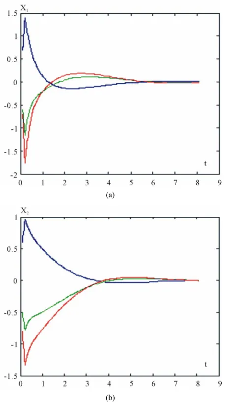
Figure 2. Numerical solutions if example 2, x1 component (a)

and x2 component (b).

Example 2

 

2

1 f t

t

 ,

 

1 e t2 , t

 _{ } 





1 2

1 , ,1 2 2

x x g t x x

t

 and







12 22



2 2 , ,1 2

x x

t

 .

g t x x 

We solved these two examples numerically using th order Runge-Kutta method. The results of example 1 are drawn as shown in Figure 1 and the results of

exam-own in Figure 2. The curves are rawn for different initial values of

d 2 demonstrate time increases all the comp ents of the solutions tends to zero. means, that t e a ptotically stable. W verify the rightness of our proved theorems.

4. Conclusion

ifo ly stable as well as

REFERENCES

nd T. Furumochi, “A Note on Stability by

87.

[4] J. Hale, “Ordina ,” Wiley Inter- science, John W oken, 1969.

four-

ple 2 are drawn as sh

d x0.

that, as the Figures 1 an

on This

he solutions ar sym hich

We introduced two theorems which provide the sufficient conditions for the boundedness of solution of the nonlinear damped vectorial oscillator and the conditions for the stability of the zero solution to be un rm

asymptotically stable. We verified our theoretical results by solving two examples satisfying the assumptions of the two proved theorems.

[1] T. A. Burton a

Schauder’s Theorem,” Funkcialaj Ekvacioj, Vol. 44, No.

1, 2001, pp. 73-82.

[2] V. A. Coppel, “Stability and Asymptotic Behavior of Dif- ferential Equations,” D. C. Heath and Company, Lexing- ton, 1965.

[3] D. Grossman, “Introduction to Differential Equations with Boundary Value Problems,” Wiley-Interscience, John Wiley & Sons, Inc., Hoboken, 19

ry Differential Equations iley & Sons, Inc., Hob

[5] G. H. Moroşanu and C. Vladimirescu, “Stability for a Non- linear Second Order ODE,” Funkcialaj Ekvacioj,Vol. 48, No. 1, 2005, pp. 49-56. doi:10.1619/fesi.48.49

[6] G. H. Moroşanu and C. Vladimirescu, “Stability for a Damped Nonlinear Oscillator,” Nonlinear Analysis, Vol. 60, No. 2, 2005, pp. 303-310.

[7] J. Awrejcewicz, “Classical Mechanics. Dynamics,” Sprin- ger-Verlag, New York, 2012,

[8] R. F. Curtain and A. J. Pritchard, “Functional Analysis in

l and Inte- Modern Applied Mathematics,” Academic Press Inc. Ltd., London, 1977.

[9] R. Bellman, “Stability Theory of Differential Equations,” Dover Publications Inc., Mineola, 1953.

[10] V. Lakshmikantham and S. Leela, “Differentia

[image:5.595.60.300.83.492.2]