Learning Word Like Units from Joint Audio Visual Analysis

Proceedings of the 55th Annual Meeting of the Association for Computational Linguistics, pages 506–517

Proceedings of the 55th Annual Meeting of the Association for Computational Linguistics, pages 506–517

Learning word-like units from joint audio-visual analysis

David Harwath and James Glass

Computer Science and Artificial Intelligence Laboratory Massachusetts Institute of Technology

Cambridge, MA 02139, USA

{dharwath,glass_}@mit.edu

Abstract

Given a collection of images and spoken audio captions, we present a method for discovering word-like acoustic units in the continuous speech signal and grounding them to semantically relevant image re-gions. For example, our model is able to detect spoken instances of the words “lighthouse” within an utterance and as-sociate them with image regions contain-ing lighthouses. We do not use any form of conventional automatic speech recog-nition, nor do we use any text transcrip-tions or conventional linguistic annota-tions. Our model effectively implements a form of spoken language acquisition, in which the computer learns not only to rec-ognize word categories by sound, but also to enrich the words it learns with seman-tics by grounding them in images.

1 Introduction

1.1 Problem Statement and Motivation

Automatically discovering words and other el-ements of linguistic structure from continuous speech has been a longstanding goal in com-putational linguists, cognitive science, and other speech processing fields. Practically all humans acquire language at a very early age, but this task has proven to be an incredibly difficult problem for computers. While conventional automatic speech recognition (ASR) systems have a long history and have recently made great strides thanks to the vival of deep neural networks (DNNs), their re-liance on highly supervised training paradigms has essentially restricted their application to the ma-jor languages of the world, accounting for a small fraction of the more than 7,000 human languages spoken worldwide (Lewis et al.,2016). The main

reason for this limitation is the fact that these su-pervised approaches require enormous amounts of very expensive human transcripts. Moreover, the use of the written word is a convenient but limiting convention, since there are many oral languages which do not even employ a writing system. In constrast, infants learn to communicate verbally before they are capable of reading and writing - so there is no inherent reason why spoken language systems need to be inseparably tied to text.

The key contribution of this paper has two facets. First, we introduce a methodology capable of not only discovering word-like units from con-tinuous speech at the waveform level with no ad-ditional text transcriptions or conventional speech recognition apparatus. Instead, we jointly learn the semantics of those units via visual associa-tions. Although we evaluate our algorithm on an English corpus, it could conceivably run on any language without requiring any text or associated ASR capability. Second, from a computational perspective, our method of speech pattern discov-ery runs in linear time. Previous work has pre-sented algorithms for performing acoustic pattern discovery in continuous speech (Park and Glass, 2008;Jansen et al.,2010;Jansen and Van Durme, 2011) without the use of transcriptions or another modality, but those algorithms are limited in their ability to scale by their inherentO(n2₎ complex-ity, since they do an exhaustive comparison of the data against itself. Our method leverages corre-lated information from a second modality - the vi-sual domain - to guide the discovery of words and phrases. This enables our method to run inO(n)

time, and we demonstrate it scalability by discov-ering acoustic patterns in over 522 hours of audio.

1.2 Previous Work

A sub-field within speech processing that has garnered much attention recently is unsupervised

speech pattern discovery. Segmental Dynamic Time Warping (S-DTW) was introduced by Park and Glass (2008), which discovers repetitions of the same words and phrases in a collection of un-transcribed acoustic data. Many subsequent ef-forts extended these ideas (Jansen et al., 2010; Jansen and Van Durme,2011;Dredze et al.,2010; Harwath et al., 2012; Zhang and Glass, 2009). Alternative approaches based on Bayesian non-parametric modeling (Lee and Glass, 2012; On-del et al., 2016) employed a generative model to cluster acoustic segments into phoneme-like categories, and related works aimed to segment and cluster either reference or learned phoneme-like tokens into higher-level units (Johnson,2008; Goldwater et al.,2009;Lee et al.,2015).

While supervised object detection is a stan-dard problem in the vision community, several re-cent works have tackled the problem of weakly-supervised or unweakly-supervised object localization (Bergamo et al., 2014; Cho et al., 2015; Zhou et al.,2015;Cinbis et al.,2016). Although the fo-cus of this work is discovering acoustic patterns, in the process we jointly associate the acoustic patterns with clusters of image crops, which we demonstrate capture visual patterns as well.

The computer vision and NLP communities have begun to leverage deep learning to create multimodal models of images and text. Many works have focused on generating annotations or text captions for images (Socher and Li, 2010; Frome et al.,2013;Socher et al.,2014;Karpathy et al.,2014;Karpathy and Li,2015;Vinyals et al., 2015;Fang et al.,2015;Johnson et al.,2016). One interesting intersection between word induction from phoneme strings and multimodal modeling of images and text is that ofGelderloos and Chru-paa (2016), who uses images to segment words within captions at the phoneme string level. Other work has taken these ideas beyond text, and at-tempted to relate images to spoken audio captions directly at the waveform level (Roy, 2003; Har-wath and Glass,2015;Harwath et al.,2016). The work of (Harwath et al.,2016) is the most similar to ours, in which the authors learned embeddings at the entire image and entire spoken caption level and then used the embeddings to perform bidirec-tional retrieval. In this work, we go further by au-tomatically segmenting and clustering the spoken captions into individual word-like units, as well as the images into object-like categories.

2 Experimental Data

We employ a corpus of over 200,000 spoken cap-tions for images taken from the Places205 dataset (Zhou et al., 2014), corresponding to over 522 hours of speech data. The captions were col-lected using Amazon’s Mechanical Turk service, in which workers were shown images and asked to describe them verbally in a free-form manner. The data collection scheme is described in detail in Harwath et al. (2016), but the experiments in this paper leverage nearly twice the amount of data. For training our multimodal neural network as well as the pattern discovery experiments, we use a subset of 214,585 image/caption pairs, and we hold out a set of 1,000 pairs for evaluating the multimodal network’s retrieval ability. Because we lack ground truth text transcripts for the data, we used Google’s Speech Recognition public API to generate proxy transcripts which we use when analyzing our system. Note that the ASR was only used for analysis of the results, and was not in-volved in any of the learning.

3 Audio-Visual Embedding Neural Networks

filterbanks with a 25ms Hamming window and a 10ms shift. The input to this branch always has 1 color channel and is always 40 pixels high (corresponding to the 40 Mel filterbanks), but the width of the spectrogram varies depending upon the duration of the spoken caption, with each pixel corresponding to approximately 10 milliseconds worth of audio. The architecture we use is entirely convolutional and shown below, where C denotes the number of convolutional channels, W is filter width, H is filter height, and S is pooling stride.

1. Convolution: C=128, W=1, H=40, ReLU 2. Convolution: C=256, W=11, H=1, ReLU 3. Maxpool: W=3, H=1, S=2

4. Convolution: C=512, W=17, H=1, ReLU 5. Maxpool: W=3, H=1, S=2

6. Convolution: C=512, W=17, H=1, ReLU 7. Maxpool: W=3, H=1, S=2

8. Convolution: C=1024, W=17, H=1, ReLU 9. Meanpool over entire caption

10. L2 normalization

In practice during training, we restrict the cap-tion spectrograms to all be 1024 frames wide (i.e., 10sec of speech) by applying truncation or zero padding. Additionally, both the images and spec-trograms are mean normalized before training. The overall multimodal network is formed by ty-ing together the image and audio branches with a layer which takes both of their output vectors and computes an inner product between them, repre-senting the similarity score between a given im-age/caption pair. We train the network to assign high scores to matching image/caption pairs, and lower scores to mismatched pairs.

Within a minibatch of B image/caption pairs, letS_jp,j = 1, . . . , Bdenote the similarity score of

thejthimage/caption pair as output by the neural

network. Next, for each pair we randomly sam-ple one impostor caption and one impostor image from the same minibatch. LetS_ji denote the

simi-larity score between thejth_{caption and its} impos-tor image, andS_jcbe the similarity score between

thejth_{image and its impostor caption. The total} loss for the entire minibatch is then computed as

L(θ) =

B X

j=1

[max(0, S_jc₋S_jp+ 1)

+ max(0, S_ji−S_jp+ 1)] (1)

We train the neural network with 50 epochs of stochastic gradient descent using a batch sizeB =

128, a momentum of 0.9, and a learning rate of 1e-5 which is set to geometrically decay by a factor between 2 and 5 every 5 to 10 epochs.

4 Finding and Clustering Audio-Visual Caption Groundings

Although we have trained our multimodal network to compute embeddings at the granularity of entire images and entire caption spectrograms, we can easily apply it in a more localized fashion. In the case of images, we can simply take any arbitrary crop of an original image and resize it to 224x224 pixels. The audio network is even more trivial to apply locally, because it is entirely convolutional and the final mean pooling layer ensures that the output will be a 1024-dim vector no matter the extent of the input. The bigger question iswhere to locally apply the networks in order to discover meaningful acoustic and visual patterns.

Given an image and its corresponding spoken audio caption, we use the term grounding to refer to extracting meaningful segments from the cap-tion and associating them with an appropriate sub-region of the image. For example, if an image depicted a person eating ice cream and its cap-tion contained the spoken words “A person is en-joying some ice cream,” an ideal set of ground-ings would entail the acoustic segment contain-ing the word “person” linked to a boundcontain-ing box around the person, and the segment containing the word “ice cream” linked to a box around the ice cream. We use a constrained brute force ranking scheme to evaluate all possible groundings (with a restricted granularity) between an image and its caption. Specifically, we divide the image into a grid, and extract all of the image crops whose boundaries sit on the grid lines. Because we are mainly interested in extracting regions of interest and not high precision object detection boxes, to keep the number of proposal regions under con-trol we impose several restrictions. First, we use a 10x10 grid on each image regardless of its original size. Second, we define minimum and maximum aspect ratios as 2:3 and 3:2 so as not to introduce too much distortion and also to reduce the num-ber of proposal boxes. Third, we define a mini-mum bounding width as 30% of the original image width, and similarly a minimum height as 30% of the original image height. In practice, this results in a few thousand proposal regions per image.

caption spectrogram, we similarly define a 1-dim grid along the time axis, and consider all possible start/end points at 10 frame (pixel) intervals. We impose minimum and maximum segment length constraints at 50 and 100 frames (pixels), implying that our discovered acoustic patterns are restricted to fall between 0.5 and 1 second in duration. The number of proposal segments will vary depend-ing on the caption length, and typically number in the several thousands. Note that when learn-ing groundlearn-ings we consider the entire audio se-quence, and do not incorporate the 10sec duration constraint imposed during training.

Once we have extracted a set of proposed visual bounding boxes and acoustic segments for a given image/caption pair, we use our multimodal net-work to compute a similarity score between each unique image crop/acoustic segment pair. Each triplet of an image crop, acoustic segment, and similarity score constitutes a proposed grounding. A naive approach would be to simply keep the top

N groundings from this list, but in practice we

ran into two problems with this strategy. First, many proposed acoustic segments capture mostly silence due to pauses present in natural speech. We solve this issue by using a simple voice activity de-tector (VAD) which was trained on the TIMIT cor-pus(Garofolo et al.,1993). If the VAD estimates that 40% or more of any proposed acoustic seg-ment is silence, we discard that entire grounding. The second problem we ran into is the fact that the top of the sorted grounding list is dominated by highly overlapping acoustic segments. This makes sense, because highly informative content words will show up in many different groundings with slightly perturbed start or end times. To allevi-ate this issue, when evaluating a grounding from the top of the proposal list we compare the in-terval intersection over union (IOU) of its acous-tic segment against all acousacous-tic segments already accepted for further consideration. If the IOU exceeds a threshold of 0.1, we discard the new grounding and continue moving down the list. We stop accumulating groundings once the scores fall to below 50% of the top score in the “keep” list, or when 10 groundings have been added to the “keep” list. Figure1displays a pictorial example of our grounding procedure.

Once we have completed the grounding proce-dure, we are left with a small set of regions of interest in each image and caption spectrogram.

We use the respective branches of our multimodal network to compute embedding vectors for each grounding’s image crop and acoustic segment. We then employk-means clustering separately on the collection of image embedding vectors as well as the collection of acoustic embedding vectors. The last step is to establish an affinity score between each image clusterIand each acoustic clusterA; we do so using the equation

Affinity(_I,_A) =X i∈I

X

a∈A

i>a_·Pair(i,a) (2)

whereiis an image crop embedding vector,ais an acoustic segment embedding vector, and Pair(i,a)

is equal to 1 when i and a belong to the same

grounding pair, and 0 otherwise. After clustering, we are left with a set of acoustic pattern clusters, a set of visual pattern clusters, and a set of linkages describing which acoustic clusters are associated with which image clusters. In the next section, we investigate these clusters in more detail.

5 Experiments and Analysis

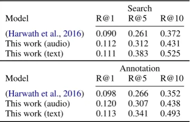
Table 1: Results for image search and annotation on the Places audio caption data (214k training pairs, 1k testing pairs). Recall is shown for the top 1, 5, and 10 hits. The model we use in this paper is compared against the meanpool variant of the model architecture presented inHarwath et al. (2016). For both training and testing, the captions were truncated/zero-padded to 10 seconds.

Search

Model R@1 R@5 R@10

(Harwath et al.,2016) 0.090 0.261 0.372 This work (audio) 0.112 0.312 0.431 This work (text) 0.111 0.383 0.525

Annotation

Model R@1 R@5 R@10

(Harwath et al.,2016) 0.098 0.266 0.352 This work (audio) 0.120 0.307 0.438 This work (text) 0.113 0.341 0.493

Figure 1: An example of our grounding method. The left image displays a grid defining the allowed start and end coordinates for the bounding box proposals. The bottom spectrogram displays several audio region proposals drawn as the families of stacked red line segments. The image on the right and spectrogram on the top display the final output of the grounding algorithm. The top spectrogram also displays the time-aligned text transcript of the caption, so as to demonstrate which words were captured by the groundings. In this example, the top 3 groundings have been kept, with the colors indicating the audio segment which is grounded to each bounding box.

Word Count Word Count

ocean 2150 castle 766 (silence) 127 (silence) 70 the ocean 72 capital 39 blue ocean 29 large castle 24 body ocean 22 castles 23

oceans 16 (noise) 21

ocean water 16 council 13 (noise) 15 stone castle 12 of ocean 14 capitol 10 oceanside 14 old castle 10

Table 2: Examples of the breakdown of word/phrase identities of several acoustic clusters

achieved by a model which uses the ASR text tran-scriptions for each caption instead of the speech audio. The text captions were truncated/padded to 20 words, and the audio branch of the network was replaced with a branch with the following ar-chitecture:

1. Word embedding layer of dimension 200

2. Temporal Convolution: C=512, W=3, ReLU 3. Temporal Convolution: C=1024, W=3 4. Meanpool over entire caption

5. L2 normalization

One would expect that access to ASR hypotheses should improve the recall scores, but the perfor-mance gap is not enormous. Access to the ASR hypotheses provides a relative improvement of ap-proximately 21.8% for image search R@10 and 12.5% for annotation R@10 compared to using no transcriptions or ASR whatsoever.

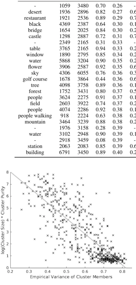
Table 3: Top 50 clusters withk = 500 sorted by increasing variance. Legend: _|Cc|is acoustic cluster size,|Ci|is associated image cluster size, Pur. is acoustic cluster purity,σ2 is acoustic cluster variance, and Cov. is acoustic cluster coverage. A dash (-) indicates a cluster whose majority label is silence.

Trans |Cc| |Ci| Pur. σ2 Cov. Trans |Cc| |Ci| Pur. σ2 Cov.

- 1059 3480 0.70 0.26 - snow 4331 3480 0.85 0.26 0.45

desert 1936 2896 0.82 0.27 0.67 kitchen 3200 2990 0.88 0.28 0.76 restaurant 1921 2536 0.89 0.29 0.71 mountain 4571 2768 0.86 0.30 0.38 black 4369 2387 0.64 0.30 0.17 skyscraper 843 3205 0.84 0.30 0.84

bridge 1654 2025 0.84 0.30 0.25 tree 5303 3758 0.90 0.30 0.16

castle 1298 2887 0.72 0.31 0.74 bridge 2779 2025 0.81 0.32 0.41

- 2349 2165 0.31 0.33 - ocean 2913 3505 0.87 0.33 0.71

table 3765 2165 0.94 0.33 0.23 windmill 1458 3752 0.71 0.33 0.76

window 1890 2795 0.85 0.34 0.21 river 2643 3204 0.76 0.35 0.62

water 5868 3204 0.90 0.35 0.27 beach 1897 2964 0.79 0.35 0.64

flower 3906 2587 0.92 0.35 0.67 wall 3158 3636 0.84 0.35 0.23

sky 4306 6055 0.76 0.36 0.34 street 2602 2385 0.86 0.36 0.49

golf course 1678 3864 0.44 0.36 0.63 field 3896 3261 0.74 0.36 0.37 tree 4098 3758 0.89 0.36 0.13 lighthouse 1254 1518 0.61 0.36 0.83 forest 1752 3431 0.80 0.37 0.56 church 2503 3140 0.86 0.37 0.72 people 3624 2275 0.91 0.37 0.14 baseball 2777 1929 0.66 0.37 0.86

field 2603 3922 0.74 0.37 0.25 car 3442 2118 0.79 0.38 0.27

people 4074 2286 0.92 0.38 0.17 shower 1271 2206 0.74 0.38 0.82 people walking 918 2224 0.63 0.38 0.25 wooden 3095 2723 0.63 0.38 0.28

mountain 3464 3239 0.88 0.38 0.29 tree 3676 2393 0.89 0.39 0.11

- 1976 3158 0.28 0.39 - snow 2521 3480 0.79 0.39 0.24

water 3102 2948 0.90 0.39 0.14 rock 2897 2967 0.76 0.39 0.26

- 2918 3459 0.08 0.39 - night 3027 3185 0.44 0.39 0.59

station 2063 2083 0.85 0.39 0.62 chair 2589 2288 0.89 0.39 0.22 building 6791 3450 0.89 0.40 0.21 city 2951 3190 0.67 0.40 0.50

Figure 2: Scatter plot of audio cluster purity weighted by log cluster size vs variance for k = 500(least-squares line superimposed).

based on the standard WSJ recipe and trained us-ing the Google ASR hypothesis as a proxy for the transcriptions. Any word whose duration is over-lapped 30% or more by the acoustic segment is in-cluded in the label string for the segment. We then employ a majority vote scheme to derive the over-all cluster labels. When computing the purity of a

cluster, we count a cluster member as matching the cluster label as long as the overall cluster label ap-pears in the member’s label string. In other words, an acoustic segment overlapping the words “the lighthouse” would receive credit for matching the overall cluster label “lighthouse”. A breakdown of the segments captured by two clusters is shown in Table2. We investigated some simple schemes for predicting highly pure clusters, and found that the empirical variance of the cluster members (aver-age squared distance to the cluster centroid) was a good indicator. Figure2displays a scatter plot of cluster purity weighted by the natural log of the cluster size against the empirical variance. Large, pure clusters are easily predicted by their low em-pirical variance, while a high variance is indicative of a garbage cluster.

Ranking a set of k = 500acoustic clusters by

clus-sky grass sunset ocean river

castle couch wooden lighthouse train

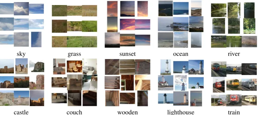
Figure 3: The 9 most central image crops from several image clusters, along with the majority-vote label of their most associated acoustic pattern cluster

Table 4: Clustering statistics of the acoustic clusters for various values ofkand different settings of the

variance-based cluster pruning threshold. Legend:|C|= number of clusters remaining after pruning,|X |

= number of datapoints after pruning, Pur = purity,|L|= number of unique cluster labels, AC = average cluster coverage

σ2_{<0.9 σ}2_<0.65

k _{|C| |X |} Pur |L| AC |C| |X | Pur |L| AC

250 249 1081514 .364 149 .423 128 548866 .575 108 .463 500 499 1097225 .396 242 .332 278 623159 .591 196 .375 750 749 1101151 .409 308 .406 434 668771 .585 255 .450 1000 999 1103391 .411 373 .336 622 710081 .568 318 .382 1500 1496 1104631 .429 464 .316 971 750162 .566 413 .366 2000 1992 1106418 .431 540 .237 1354 790492 .546 484 .271

ter label anywhere in the training data, and then compute what fraction of those instances were captured by the cluster. There are many examples of high coverage clusters, e.g. the “skyscraper” cluster captures 84% of all occurrences of the word “skyscraper”, while the “baseball” cluster captures 86% of all occurrences of the word “base-ball”. This is quite impressive given the fact that no conventional speech recognition was em-ployed, and neither the multimodal neural network nor the grounding algorithm had access to the text transcripts of the captions.

To get an idea of the impact of thekparameter

as well as a variance-based cluster pruning thresh-old based on Figure 2, we swept k from 250 to

2000 and computed a set of statistics shown in Table 4. We compute the standard overall clus-ter purity evaluation metric in addition to the aver-age coveraver-age across clusters. The table shows the natural tradeoff between cluster purity and

redun-dancy (indicated by the average cluster coverage) askis increased. In all cases, the variance-based

cluster pruning greatly increases both the overall purity and average cluster coverage metrics. We also notice that more unique cluster labels are dis-covered with a largerk.

Next, we examine the image clusters. Figure 3 displays the 9 most central image crops for a set of 10 different image clusters, along with the majority-vote label of each image cluster’s asso-ciated audio cluster. In all cases, we see that the image crops are highly relevant to their audio clus-ter label. We include many more example image clusters in Appendix A.

In order to examine the semantic embedding space in more depth, we took the top 150 clusters from the same k = 500clustering run described

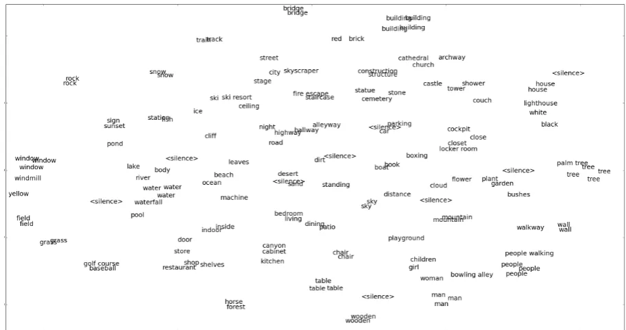
di-Figure 4: t-SNE analysis of the 150 lowest-variance audio pattern cluster centroids fork = 500.

Dis-played is the majority-vote transcription of the each audio cluster. All clusters shown contained a mini-mum of 583 members and an average of 2482, with an average purity of .668.

mensions and plotted their majority-vote labels in Figure4. Immediately we see that different clus-ters which capture the same label closely neigh-bor one another, indicating that distances in the embedding space do indeed carry information dis-criminative across word types (and suggesting that a more sophisticated clustering algorithm thank

-means would perform better). More interestingly, we see that semantic information is also reflected in these distances. The cluster centroids for “lake,” “river,” “body,” “water,” “waterfall,” “pond,” and “pool” all form a tight meta-cluster, as do “restau-rant,” “store,” “shop,” and “shelves,” as well as “children,” “girl,” “woman,” and “man.” Many other semantic meta-clusters can be seen in Figure 4, suggesting that the embedding space is captur-ing information that is highly discriminative both acousticallyandsemantically.

Because our experiments revolve around the discovery of word and object categories, a key question to address is the extent to which the supervision used to train the VGG network constrains or influences the kinds of objects learned. Because the 1,000 object classes from the ILSVRC2012 task (Russakovsky et al.,2015) used to train the VGG network were derived from WordNet synsets (Fellbaum,1998), we can mea-sure the semantic similarity between the words

learned by our network and the ILSVRC2012 class labels by using synset similarity measures within WordNet. We do this by first building a list of the 1,000 WordNet synsets associated with the ILSVRC2012 classes. We then take the set of unique majority-vote labels associated with the discovered word clusters fork = 500, filtered by

setting a threshold on their variance (σ2 _≤ 0.65)

other words, more than two thirds of the highly pure pattern clusters learned by our network were dissimilar to all of the 1,000 ILSVRC12 classes used to pretrain the VGG network, indicating that our model is able to generalize far beyond the set of classes found in the ILSVRC12 data. We dis-play the labels of the 40 lowest variance acoustic clusters labels along with the name and similarity score of their closest ILSVRC12 synset in Table5.

Cluster ILSVRC synset Similarity

snow cliff.n.01 0.14

desert cliff.n.01 0.12

kitchen patio.n.01 0.25

restaurant restaurant.n.01 1.00

mountain alp.n.01 0.50

black pool table.n.01 0.25

skyscraper greenhouse.n.01 0.33 bridge steel arch bridge.n.01 0.50

tree daisy.n.01 0.14

castle castle.n.02 1.00

ocean cliff.n.01 0.14

table desk.n.01 0.50

windmill cash machine.n.01 0.20

window screen.n.03 0.33

river cliff.n.01 0.12

water menu.n.02 0.25

beach cliff.n.01 0.33

flower daisy.n.01 0.50

wall cliff.n.01 0.33

sky cliff.n.01 0.11

street swing.n.02 0.14

golf course swing.n.02 0.17

field cliff.n.01 0.20

lighthouse beacon.n.03 1.00

forest cliff.n.01 0.20

church church.n.02 1.00

people street sign.n.01 0.17

baseball baseball.n.02 1.00

car freight car.n.01 0.50

shower swing.n.02 0.17

people walking (none) 0.00

wooden (none) 0.00

rock toilet tissue.n.01 0.20

night street sign.n.01 0.14

station swing.n.02 0.20

chair barber chair.n.01 0.50 building greenhouse.n.01 0.50

city cliff.n.01 0.12

white jean.n.01 0.33

sunset street sign.n.01 0.11

Table 5: The 40 lowest variance, uniquely-labeled acoustic clusters paired with their most similar ILSVRC2012 synset.

6 Conclusions and Future Work

In this paper, we have demonstrated that a neu-ral network trained to associate images with the waveforms representing their spoken audio cap-tions can successfully be applied to discover and

cluster acoustic patterns representing words or short phrases in untranscribed audio data. An analogous procedure can be applied to visual im-ages to discover visual patterns, and then the two modalities can be linked, allowing the network to learn, for example, that spoken instances of the word “train” are associated with image re-gions containing trains. This is done without the use of a conventional automatic speech recogni-tion system and zero text transcriprecogni-tions, and there-fore is completely agnostic to the language in which the captions are spoken. Further, this is done in O(n) time with respect to the number

of image/caption pairs, whereas previous state-of-the-art acoustic pattern discovery algorithms which leveraged acoustic data alone run inO(n2₎ time. We demonstrate the success of our method-ology on a large-scale dataset of over 214,000 im-age/caption pairs comprising over 522 hours of spoken audio data, which is to our knowledge the largest scale acoustic pattern discovery exper-iment ever performed. We have shown that the shared multimodal embedding space learned by our model is discriminative not only across visual object categories, but also acousticallyand seman-tically across spoken words.

References

Alessandro Bergamo, Loris Bazzani, Dragomir Anguelov, and Lorenzo Torresani. 2014. Self-taught object lo-calization with deep networks. CoRR abs/1409.3964.

http://arxiv.org/abs/1409.3964.

Minsu Cho, Suha Kwak, Cordelia Schmid, and Jean Ponce. 2015. Unsupervised object discovery and localization in the wild: Part-based matching with bottom-up region pro-posals. InProceedings of CVPR.

Ramazan Cinbis, Jakob Verbeek, and Cordelia Schmid. 2016. Weakly supervised object localization with multi-fold multiple instance learning. InIEEE Transactions on Pat-tern Analysis and Machine Intelligence.

Mark Dredze, Aren Jansen, Glen Coppersmith, and Kenneth Church. 2010. NLP on spoken documents without ASR. InProceedings of EMNLP.

Hao Fang, Saurabh Gupta, Forrest Iandola, Srivastava Ru-pesh, Li Deng, Piotr Dollar, Jianfeng Gao, Xiaodong He, Margaret Mitchell, Platt John C., C. Lawrence Zitnick, and Geoffrey Zweig. 2015. From captions to visual con-cepts and back. InProceedings of CVPR.

Christiane Fellbaum. 1998. WordNet: An Electronic Lexical Database. Bradford Books.

Andrea Frome, Greg S. Corrado, Jonathon Shlens, Samy Bengio, Jeffrey Dean, Marc’Aurelio Ranzato, and Tomas Mikolov. 2013. Devise: A deep visual-semantic embed-ding model. In Proceedings of the Neural Information Processing Society.

John Garofolo, Lori Lamel, William Fisher, Jonathan Fiscus, David Pallet, Nancy Dahlgren, and Victor Zue. 1993. The TIMIT acoustic-phonetic continuous speech corpus. Lieke Gelderloos and Grzegorz Chrupaa. 2016. From

phonemes to images: levels of representation in a recur-rent neural model of visually-grounded language learning. InarXiv:1610.03342.

Sharon Goldwater, Thomas Griffiths, and Mark Johnson. 2009. A Bayesian framework for word segmentation: exploring the effects of context. InCognition, vol. 112 pp.21-54.

David Harwath and James Glass. 2015. Deep multimodal semantic embeddings for speech and images. In Proceed-ings of the IEEE Workshop on Automatic Speech Recogni-tion and Understanding.

David Harwath, Timothy J. Hazen, and James Glass. 2012. Zero resource spoken audio corpus analysis. In Proceed-ings of ICASSP.

David Harwath, Antonio Torralba, and James R. Glass. 2016. Unsupervised learning of spoken language with visual context. InProceedings of NIPS.

Aren Jansen, Kenneth Church, and Hynek Hermansky. 2010. Toward spoken term discovery at scale with zero re-sources. InProceedings of Interspeech.

Aren Jansen and Benjamin Van Durme. 2011. Efficient spo-ken term discovery using randomized algorithms. In Pro-ceedings of IEEE Workshop on Automatic Speech Recog-nition and Understanding.

Justin Johnson, Andrej Karpathy, and Li Fei-Fei. 2016. Densecap: Fully convolutional localization networks for dense captioning. InProceedings of CVPR.

Mark Johnson. 2008. Unsupervised word segmentation for sesotho using adaptor grammars. InProceedings of ACL SIG on Computational Morphology and Phonology. Andrej Karpathy, Armand Joulin, and Fei-Fei Li. 2014. Deep

fragment embeddings for bidirectional image sentence mapping. InProceedings of the Neural Information Pro-cessing Society.

Andrej Karpathy and Fei-Fei Li. 2015. Deep visual-semantic alignments for generating image descriptions. In Proceed-ings of CVPR.

Chia-Ying Lee and James Glass. 2012. A nonparametric Bayesian approach to acoustic model discovery. In Pro-ceedings of the 2012 meeting of the Association for Com-putational Linguistics.

Chia-Ying Lee, Timothy J. O’Donnell, and James Glass. 2015. Unsupervised lexicon discovery from acoustic in-put. InTransactions of the Association for Computational Linguistics.

M. Paul Lewis, Gary F. Simon, and Charles D. Fen-nig. 2016. Ethnologue: Languages of the World, Nineteenth edition. SIL International. Online version: http://www.ethnologue.com.

Lucas Ondel, Lukas Burget, and Jan Cernocky. 2016. Vari-ational inference for acoustic unit discovery. In 5th Workshop on Spoken Language Technology for Under-resourced Language.

Alex Park and James Glass. 2008. Unsupervised pattern dis-covery in speech. InIEEE Transactions on Audio, Speech, and Language Processing vol. 16, no.1, pp. 186-197. Daniel Povey, Arnab Ghoshal, Gilles Boulianne, Lukas

Bur-get, Ondrej Glembek, Nagendra Goel, Mirko Hannemann, Petr Motlicek, Yanmin Qian, Petr Schwarz, Jan Silovsky, Georg Stemmer, and Karel Vesely. 2011. The Kaldi speech recognition toolkit. InIEEE 2011 Workshop on Automatic Speech Recognition and Understanding. Deb Roy. 2003. Grounded spoken language acquisition:

Ex-periments in word learning. InIEEE Transactions on Mul-timedia.

Olga Russakovsky, Jia Deng, Hao Su, Jonathan Krause, Sanjeev Satheesh, Sean Ma, Zhiheng Huang, Andrej Karpathy, Aditya Khosla, Michael Bernstein, Alexan-der C. Berg, and Li Fei-Fei. 2015. ImageNet Large Scale Visual Recognition Challenge. International Journal of Computer Vision (IJCV) 115(3):211–252.

https://doi.org/10.1007/s11263-015-0816-y.

Karen Simonyan and Andrew Zisserman. 2014. Very deep convolutional networks for large-scale image recognition.

CoRRabs/1409.1556.

Richard Socher and Fei-Fei Li. 2010. Connecting modalities: Semi-supervised segmentation and annotation of images using unaligned text corpora. InProceedings of CVPR. Laurens van der Maaten and Geoffrey Hinton. 2008.

Visu-alizing high-dimensional data using t-sne. InJournal of Machine Learning Research.

Oriol Vinyals, Alexander Toshev, Samy Bengio, and Dimitru Erhan. 2015. Show and tell: A neural image caption gen-erator. InProceedings of CVPR.

Yaodong Zhang and James Glass. 2009. Unsupervised spo-ken keyword spotting via segmental DTW on Gaussian posteriorgrams. InProceedings ASRU.

Bolei Zhou, Aditya Khosla, Agata Lapedriza, Aude Oliva, and Antonio Torralba. 2015. Object detectors emerge in deep scene CNNs. InProceedings of ICLR.

A Additional Cluster Visualizations

beach cliff pool desert field

chair table staircase statue stone

church forest mountain skyscraper trees

waterfall windmills window city bridge

flowers man wall archway baseball

boat shelves cockpit girl children