Word Embeddings with Limited Memory
Shaoshi Ling1and Yangqiu Song2 and Dan Roth1
1Department of Computer Science, University of Illinois at Urbana-Champaign 2Department of Computer Science and Engineering, HKUST
1{sling3,danr}@illinois.edu, 2[email protected]
Abstract
This paper studies the effect of limited pre-cision data representation and computa-tion on word embeddings. We present a systematic evaluation of word embeddings with limited memory and discuss method-s that directly train the limited precimethod-sion representation with limited memory. Our results show that it is possible to use and train an 8-bit fixed-point value for word embedding without loss of performance in word/phrase similarity and dependency parsing tasks.
1 Introduction
There is an accumulation of evidence that the use of dense distributional lexical representations, known as word embeddings, often supports bet-ter performance on a range of NLP tasks (Ben-gio et al., 2003; Turian et al., 2010; Collobert et al., 2011; Mikolov et al., 2013a; Mikolov et al., 2013b; Levy et al., 2015). Consequently, word embeddings have been commonly used in the last few years for lexical similarity tasks and as fea-tures in multiple, syntactic and semantic, NLP ap-plications.
However, keeping embedding vectors for hun-dreds of thousands of words for repeated use could take its toll both on storing the word vectors on disk and, even more so, on loading them into memory. For example, for 1 million words, load-ing 200 dimensional vectors takes up to 1.6 GB memory on a 64-bit system. Considering applica-tions that make use of billions of tokens and mul-tiple languages, size issues impose significant lim-itations on the practical use of word embeddings.
This paper presents the question of whether it is possible to significantly reduce the memory need-s for the uneed-se and training of word embeddingneed-s.
Specifically, we ask “what is the impact of repre-senting each dimension of a dense representation with significantly fewer bits than the standard64 bits?” Moreover, we investigate the possibility of directly training dense embedding vectors using significantly fewer bits than typically used.
The results we present are quite surprising. We show that it is possible to reduce the memory con-sumption by an order of magnitude both when word embeddings are being used and in training. In the first case, as we show, simply truncating the resulting representations after training and us-ing a smaller number of bits (as low as 4 bits per dimension) results in comparable performance to the use of 64 bits. Moreover, we provide t-wo ways to train existing algorithms (Mikolov et al., 2013a; Mikolov et al., 2013b) when the memory is limited during training and show that, here, too, an order of magnitude saving in mem-ory is possible without degrading performance. We conduct comprehensive experiments on ex-isting word and phrase similarity and relatedness datasets as well as on dependency parsing, to e-valuate these results. Our experiments show that, in all cases and without loss in performance, 8 bits can be used when the current standard is 64 and, in some cases, only 4 bits per dimension are sufficient, reducing the amount of space re-quired by a factor of 16. The truncated word embeddings are available from the papers web page athttps://cogcomp.cs.illinois. edu/page/publication_view/790.
2 Related Work
If we consider traditional cluster encoded word representation, e.g., Brown clusters (Brown et al., 1992), it only uses a small number of bits to track the path on a hierarchical tree of word clusters to represent each word. In fact, word embedding
generalized the idea of discrete clustering repre-sentation to continuous vector reprerepre-sentation in language models, with the goal of improving the continuous word analogy prediction and general-ization ability (Bengio et al., 2003; Mikolov et al., 2013a; Mikolov et al., 2013b). However, it has been proven that Brown clusters as discrete fea-tures are even better than continuous word em-bedding as features for named entity recognition tasks (Ratinov and Roth, 2009). Guo et al. (Guo et al., 2014) further tried to binarize embeddings using a threshold tuned for each dimension, and essentially used less than two bits to represen-t each dimension. They have shown represen-tharepresen-t bina-rization can be comparable to or even better than the original word embeddings when used as fea-tures for named entity recognition tasks. More-over, Faruqui et al. (Faruqui et al., 2015) showed that imposing sparsity constraints over the em-bedding vectors can further improve the represen-tation interpretability and performance on sever-al word similarity and text classification bench-mark datasets. These works indicate that, for some tasks, we do not need all the information encoded in “standard” word embeddings. Nonetheless, it is clear that binarization loses a lot of information, and this calls for a systematic comparison of how many bits are needed to maintain the expressivity needed from word embeddings for different tasks.
3 Value Truncation
In this section, we introduce approaches for word embedding when the memory is limited. We trun-cate any valuexin the word embedding into ann
bit representation.
3.1 Post-processing Rounding
When the word embedding vectors are given, the most intuitive and simple way is to round the num-bers to theirn-bit precision. Then we can use the truncated values as features for any tasks that word embedding can be used for. For example, if we want to round x to be in the range of [−r, r], a simple function can be applied as follows.
Rd(x, n) =
bxc if bxc ≤x≤ bxc+
2
bxc+ if bxc+
2 <x≤ bxc+
(1) where= 21−nr. For example, if we want to use
8 bits to represent any value in the vectors, then we only have 256 numbers ranging from -128 to 127
for each value. In practice, we first scale all the values and then round them to the 256 numbers.
3.2 Training with Limited Memory
When the memory for training word embedding is also limited, we need to modify the training algorithms by introducing new data structures to reduce the bits used to encode the values. In practice, we found that in the stochastic gradien-t descengradien-t (SGD) igradien-teragradien-tion in word2vec algorigradien-thm- algorithm-s (Mikolov et al., 2013a; Mikolov et al., 2013b), the updating vector’s values are often very small numbers (e.g.,<10−5). In this case, if we direct-ly appdirect-ly the rounding method to certain precisions (e.g., 8 bits), the update of word vectors will al-ways be zero. For example, the 8-bit precision is 2−7 = 0.0078, so10−5 is not significant enough to update the vector with 8-bit values. Therefore, we consider the following two ways to improve this.
Stochastic Rounding. We first consider us-ing stochastic roundus-ing (Gupta et al., 2015) to train word embedding. Stochastic rounding intro-duces some randomness into the rounding mech-anism, which has been proven to be helpful when there are many parameters in the learning system, such as deep learning systems (Gupta et al., 2015). Here we also introduce this approach to update word embedding vectors in SGD. The probability of roundingx tobxc is proportional to the prox-imity ofxtobxc:
Rs(x, n) =
bxc w.p. 1−x−bxc
bxc+ w.p. x−bxc . (2)
In this case, even though the update values are not significant enough to update the word embedding vectors, we randomly choose some of the values being updated proportional to the value of how close the update value is to the rounding precision.
Auxiliary Update Vectors. In addition to the method of directly applying rounding to the val-ues, we also provide a method using auxiliary update vectors to trade precision for more space. Suppose we know the range of update value in S-GD as [−r0, r0], and we use additional m bits to
store all the values less than the limited numeri-cal precision . Here r0 can be easily estimated
by running SGD for several examples. Then the real precision is 0 = 21−mr0. For example, if
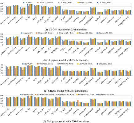
(a) CBOW model with 25 dimensions.
(b) Skipgram model with 25 dimensions.
(c) CBOW model with 200 dimensions.
[image:3.595.83.520.58.458.2](d) Skipgram model with 200 dimensions.
Figure 1:Comparing performance on multiple similarity tasks, with different values of truncation. The y-axis represents the Spearman’s rank correlation coefficient for word similarity datasets, and the cosine value for paraphrase (bigram) datasets (see Sec. 4.2).
the cumulated values in the auxiliary update vec-tors are greater than the original numerical preci-sion, e.g., = 2−7 for 8 bits, we update the o-riginal vector and clear the value in the auxiliary vector. In this case, we can have finaln-bit values in word embedding vectors as good as the method presented in Section 3.1.
4 Experiments on Word/Phrase Similarity
In this section, we describe a comprehensive study on tasks that have been used for evaluating word embeddings. We train the word embedding algo-rithms, word2vec (Mikolov et al., 2013a; Mikolov et al., 2013b), based on the Oct. 2013
Wikipedi-a dump.1 We first compare levels of truncation
of word2vec embeddings, and then evaluate the s-tochastic rounding and the auxiliary vectors based methods for training word2vec vectors.
4.1 Datasets
We use multiple test datasets as follows.
Word Similarity. Word similarity datasets have been widely used to evaluate word embed-ding results. We use the datasets summarized by Faruqui and Dyer (Faruqui and Dyer, 2014): wordsim-353, wordsim-sim, wordsim-rel, MC-30, RG-65, MTurk-287, MTurk-771, MEN 3000, YP-130, Rare-Word, Verb-143, and SimLex-999.2 We
compute the similarities between pairs of words
Table 1:The detailed average results for word similarity and paraphrases of Fig. 1. Average Original Binary CBOW4-bits 6-bits 8-bits Original Binary Skipgram4-bits 6-bits 8-bits wordsim (25) 0.5331 0.4534 0.5223 0.5235 0.5242 0.4894 0.4128 0.4333 0.4877 0.4906 wordsim (200) 0.5818 0.5598 0.4542 0.5805 0.5825 0.5642 0.5588 0.4681 0.5621 0.5637 bigram (25) 0.3023 0.2553 0.3164 0.3160 0.3153 0.3110 0.2146 0.2498 0.3050 0.3082 bigram (200) 0.3864 0.3614 0.2954 0.3802 0.3858 0.3565 0.3562 0.2868 0.3529 0.3548
and check the Spearman’s rank correlation coeffi-cient (Myers and Well., 1995) between the com-puter and the human labeled ranks.
Paraphrases (bigrams).We use the paraphrase (bigram) datasets used in (Wieting et al., 2015), ppdb all, bigrams vn, bigrams nn, and bigram-s jnn, to tebigram-st whether the truncation affectbigram-s phrabigram-se level embedding. Our phrase level embedding is based on the average of the words inside each phrase. Note that it is also easy to incorporate our truncation methods into existing phrase em-bedding algorithms. We follow (Wieting et al., 2015) in using cosine similarity to evaluate the correlation between the computed similarity and annotated similarity between paraphrases.
4.2 Analysis of Bits Needed
We ran both CBOW and skipgram with negative sampling (Mikolov et al., 2013a; Mikolov et al., 2013b) on the Wikipedia dump data, and set the window size of context to be five. Then we per-formed value truncation with 4 bits, 6 bits, and 8 bits. The results are shown in Fig. 1, and the num-bers of the averaged results are shown in Table 1. We also used the binarization algorithm (Guo et al., 2014) to truncate each dimension to three val-ues; these experiments are is denoted using the suffix “binary” in the figure. For both CBOW and skipgram models, we train the vectors with 25 and 200 dimensions respectively.
The representations used in our experiments were trained using the whole Wikipedia dump. A first observation is that, in general, CBOW per-forms better than the skipgram model. When us-ing the truncation method, the memory required to store the embedding is significantly reduced, while the performance on the test datasets remains almost the same until we truncate down to 4 bit-s. When comparing CBOW and skipgram models, we again see that the drop in performance with 4-bit values for the skipgram model is greater than the one for the CBOW model. For the CBOW model, the drop in performance with 4-bit values is greater when using 200 dimensions than it is
when using 25 dimensions. However, when using skipgram, this drop is slightly greater when using 25 dimensions than 200.
We also evaluated the binarization ap-proach (Guo et al., 2014). This model uses three values, represented using two bits. We observe that, when the dimension is 25, the bina-rization is worse than truncation. One possible explanation has to do merely with the size of the space; while325 is much larger than the size of the word space, it does not provide enough redundancy to exploit similarity as needed in the tasks. Consequently, the binarization approach results in worse performance. However, when the dimension is 200, this approach works much better, and outperforms the 4-bit truncation. In particular, binarization works better for skipgram than for CBOW with 200 dimensions. One possible explanation is that the binarization algorithm computes, for each dimension of the word vectors, the positive and negative means of the values and uses it to split the original values in that dimension, thus behaving like a model that clusters the values in each dimension. The success of the binarization then indicates that skipgram embeddings might be more discriminative than CBOW embeddings.
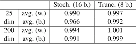
4.3 Comparing Training Methods
round-Table 2: Comparing the training CBOW models: We set the average value of the original word2vec embeddings to be 1, and the values in the table are relative to the original embeddings baselines. “avg. (w.)” represents the average values of all word similarity datasets. “avg. (b.)” represents the average values of all bigram phrase similarity datasets. “Stoch. (16 b.)” represents the method using stochastic rounding applied to 16-bit precision. “Trunc. (8 b.)” represents the method using truncation with 8-bit auxiliary update vectors applied to 8-bit precision.
Stoch. (16 b.) Trunc. (8 b.) 25 avg. (w.) 0.990 0.997 dim avg. (b.) 0.966 0.992 200 avg. (w.) 0.994 1.001 dim avg. (b.) 0.991 0.999
ing method to converge. Auxiliary update vectors achieve very similar results to the original vectors, and, in fact, result in almost the same vectors as produced by the original truncation method.
5 Experiments on Dependency Parsing We also incorporate word embedding results into a downstream task, dependency parsing, to eval-uate whether the truncated embedding results are still good features compared to the original fea-tures. We follow the setup of (Guo et al., 2015) in a monolingual setting3. We train the parser
with 5,000 iterations using different truncation set-tings for word2vec embedding. The data used to train and evaluate the parser is the English data in the CoNLL-X shared task (Buchholz and Mar-si, 2006). We follow (Guo et al., 2015) in using the labeled attachment score (LAS) to evaluate the different parsing results. Here we only show the word embedding results for 200 dimensions, since empirically we found 25-dimension results were not as stable as 200 dimensions.
The results shown in Table 3 for dependency parsing are consistent with word similarity and paraphrasing. First, we see that binarization for CBOW and skipgram is again better than the trun-cation approach. Second, for truntrun-cation results, more bits leads to better results. With 8-bits, we can again obtain results similar to those obtained
3https://github.com/jiangfeng1124/
[image:5.595.326.490.96.182.2]acl15-clnndep
Table 3: Evaluation results for dependency parsing (in LAS).
Bits CBOW Skipgram Original 88.58% 88.15%
Binary 89.25% 88.41% 4-bits 87.56% 86.46% 6-bits 88.62% 87.98% 8-bits 88.63% 88.16%
from the original word2vec embedding. 6 Conclusion
We systematically evaluated how small can the representation size of dense word embedding be before it starts to impact the performance of NLP tasks that use them. We considered both the final size of the size we provide it while learning it. Our study considers both the CBOW and the skipgram models at 25 and 200 dimensions and showed that 8 bits per dimension (and sometimes even less) are sufficient to represent each value and maintain per-formance on a range of lexical tasks. We also pro-vided two ways to train the embeddings with re-duced memory use. The natural future step is to extend these experiments and study the impact of the representation size on more advanced tasks. Acknowledgment
The authors thank Shyam Upadhyay for his help with the dependency parser embeddings results, and Eric Horn for his help with this write-up. This work was supported by DARPA under agreemen-t numbers HR0011-15-2-0025 and FA8750-13-2-0008. The U.S. Government is authorized to re-produce and distribute reprints for Governmental purposes notwithstanding any copyright notation thereon. The views and conclusions contained herein are those of the authors and should not be interpreted as necessarily representing the official policies or endorsements, either expressed or im-plied, of any of the organizations that supported the work.
References
Yoshua Bengio, R´ejean Ducharme, Pascal Vincent, and Christian Janvin. 2003. A neural probabilistic lan-guage model. Journal of Machine Learning Re-searc, 3:1137–1155.
[image:5.595.72.290.243.314.2]1992. Class-based n-gram models of natural lan-guage. Computational Linguistics, 18(4):467–479. Sabine Buchholz and Erwin Marsi. 2006. Conll-x
shared task on multilingual dependency parsing. In
CoNLL, pages 149–164.
Ronan Collobert, Jason Weston, L´eon Bottou, Michael Karlen, Koray Kavukcuoglu, and Pavel P. Kuksa. 2011. Natural language processing (almost) from scratch. Journal of Machine Learning Research, 12:2493–2537.
Manaal Faruqui and Chris Dyer. 2014. Improving vector space word representations using multilingual correlation. InEACL, pages 462–471.
Manaal Faruqui, Yulia Tsvetkov, Dani Yogatama, Chris Dyer, and Noah A. Smith. 2015. Sparse overcom-plete word vector representations. In ACL, pages 1491–1500.
Jiang Guo, Wanxiang Che, Haifeng Wang, and Ting Li-u. 2014. Revisiting embedding features for simple semi-supervised learning. In EMNLP, pages 110– 120.
Jiang Guo, Wanxiang Che, David Yarowsky, Haifeng Wang, and Ting Liu. 2015. Cross-lingual depen-dency parsing based on distributed representations. InACL, pages 1234–1244.
Suyog Gupta, Ankur Agrawal, Kailash Gopalakrish-nan, and Pritish Narayanan. 2015. Deep learning with limited numerical precision. In ICML, pages 1737–1746.
Omer Levy, Yoav Goldberg, and Ido Dagan. 2015. Im-proving distributional similarity with lessons learned from word embeddings. TACL, 3:211–225.
Tomas Mikolov, Ilya Sutskever, Kai Chen, Greg S. Cor-rado, and Jeff Dean. 2013a. Distributed representa-tions of words and phrases and their compositional-ity. InNIPS, pages 3111–3119.
Tomas Mikolov, Wen-tau Yih, and Geoffrey Zweig. 2013b. Linguistic regularities in continuous space word representations. InNAACL-HLT, pages 746– 751.
Jerome L. Myers and Arnold D. Well. 1995. Research Design & Statistical Analysisn. Routledge.
Lev Ratinov and Dan Roth. 2009. Design challenges and misconceptions in named entity recognition. In
Proceedings of CoNLL-09, pages 147–155.
Joseph Turian, Lev-Arie Ratinov, and Yoshua Bengio. 2010. Word representations: A simple and general method for semi-supervised learning. InACL, pages 384–394.