A Virtual Manipulative for Learning Log-Linear Models
Francis Ferraro and Jason Eisner Department of Computer Science
Johns Hopkins University Baltimore, MD, USA
{ferraro, jason}@cs.jhu.edu
Abstract
We present an open-source virtual ma-nipulative for conditional log-linear mod-els. This web-based interactive visual-ization lets the user tune the probabili-ties of various shapes—which grow and shrink accordingly—by dragging sliders that correspond to feature weights. The visualization displays a regularized train-ing objective; it supports gradient as-cent by optionally displaying gradients on the sliders and providing “Step” and “Solve” buttons. The user can sam-ple parameters and datasets of differ-ent sizes and compare their own pa-rameters to the truth. Our web-site,http://cs.jhu.edu/˜jason/ tutorials/loglin/, guides the user through a series of interactive lessons and provides auxiliary readings, explanations, practice problems and resources.
1 Introduction
We argue that if one is going to teach only a sin-gle machine learning technique in a computational linguistics course, it should be conditional log-linear modeling. Such models are pervasive in nat-ural language processing. They have the form
p~θ(y|x)∝exp
~
θ·f~(x, y)
, (1)
where f~extracts a feature vector from contextx
and outcomey ∈ Y(x). The set of possible out-comesY(x)might depend on the contextx.1
1The model is equivalent to logistic regression whenyis
a binary variable, that is, whenY(x) ={0,1}.
We then present an interactive web visualiza-tion that guides students through playing with log-linear models and their estimation. This open-source tool, available at http://cs.jhu. edu/˜jason/tutorials/loglin/, is in-tended to develop intuitions, so that basic log-linear models can be then taken for granted in fu-ture lecfu-tures. It can be used near the start of a course, perhaps after introducing probability no-tation andn-gram models.
We used the tool in our Natural Language Pro-cessing (NLP) class and received very positive feedback. Students were excited by it, with some saying the tool helped develop their “physical in-tuition” for log-linear models. Other test users with no technical background also enjoyed work-ing through the introductory lessons and found that they began to understand the model.
The app includes 18 ready-to-use lessons for in-dividual or small-group study or classroom use. Each lesson, e.g. Figure 1, guides the student to fit a probability modelp~θ(y|x)over some collec-tion Y of shapes, words, or other images such as parse trees. Each lesson is peppered with ques-tions; students can be asked to answer some of these questions in writing.2 Ambitious instruc-tors can add new lessons or edit existing ones by writing configuration files (see section 5.3). This is useful for emphasizing specific concepts or ap-plications. Section 8 provides some history and applications of log-linear modeling, as well as as-signment ideas.
2There are approximately 6 questions per lesson. We
found that answeringallthe questions took our students about 2300 words, or just under 23 words per question, which was probably both unreasonable and unnecessary.
Figure 1: The first lesson; the lower half is larger on the actual application.
2 Why Teach With Log-Linear Models?
Log-linear models are very handy in NLP. They can be usedthroughouta course, when one needs
• a global classifier for an applied task, such as detecting sentiment, topic, spam, or gender;
• a local classifier for structure annotation, such as tags or segment boundaries;
• a local classifier to be applied repeatedly in sequential decision-making;
• a local conditional probability within some generative process, such as ann-gram model, HMM, PCFG, probabilistic FSA or FST, noisy-channel MT model, or Bayes net;
• a global structured prediction method. Here
y is a complete structured object such as a tagging, segmentation, parse, alignment, or translation. Thenp(y | x) is a Markov ran-dom field or a conditional ranran-dom field, de-pending on whetherxis empty or not.
Log-linear models over discrete variables are also sufficiently expressive for an NLP course.
Students may experiment freely with adding their own creative modelfeaturesthat refer to salient at-tributesorpropertiesof the data, since the proba-bility (1) may consider any number of informative features of the(x, y)pair.
How about training? Estimation of the pa-rameter weights ~θ from a set of fully observed (x, y)pairs is simply a convex optimization prob-lem. Maximizing the regularized conditional log-likelihood
F(~θ) = N
X
i=1
logp~θ(yi | xi)
!
−C·R(θ~) (2)
log-linear models, including, among others, MegaM (Daum´e III, 2004), and NLTK (Bird et al., 2009).3 Formally, log-linear models are a good gate-way to a more general understanding of undirected graphical models and the exponential family, in-cluding globally normalized joint or conditional distributions over trees and sequences.
One reason that log-linear models are both ver-satile and pedagogically useful is that they do not just make predictions, but explicitly model proba-bilities. These can be
• combined with other probabilities using the usual rules of probability;
• marginalized at test time to obtain the prob-ability that the outcome y has a particular property (e.g., one can sum over alignments);
• marginalized at training time in the case of incomplete datay(e.g., the training data may not include alignments);
• used to choose among possible decisions by computing their expected loss (risk).
The training procedure also takes a probabilis-tic view. Equation (2) helps illustrate impor-tant statistical principles such as maximum likeli-hood,4 regularization (the bias-variance tradeoff), and cross-validation, as well as optimization prin-ciples such as gradient ascent.
Log-linear models also provide natural exten-sions of commonly taught NLP methods. For ex-ample, under a probabilistic context-free gram-mar (PCFG),5 p(parse tree | sentence)is propor-tional to a product of rule probabilities. Simply replacing each rule probability with an arbitrary non-negativepotential—an exponentiated weight, or sum of weights of features of that rule—gives an instance of (1). The same parsing algorithms still apply without modification, as does the same inside-outside approach to computing the poste-rior expectation of rule counts and feature counts. Immediate variants include CRF CFGs (Finkel
3
A caveat is that generic log-linear training tools will iter-ateover the setY(x)in order to maximize (1) and to compute the constant of proportionality in (1) and the gradient of (2). This is impractical whenY(x)is large, as in language mod-eling or structured prediction. See Section 8.
4Historically, this objective has been regarded as the
opti-mization dual of a maximum entropy problem (Berger et al., 1996), motivating the log-linear form of (2). We have consid-ered adding a maximum entropy view to our manipulative.
5Likewise for Markov or hidden Markov models.
et al., 2008), in which the rule features become position-dependent and sentence-dependent, and log-linear PCFGs (Berg-Kirkpatrick et al., 2010), in which the feature-rich rule potentials are locally renormalized into rule probabilities via (1).
For all these reasons, we recommend log-linear models as one’s “go-to” machine learning tech-nique when teaching. Other linear classifiers, such as perceptrons and SVMs, similarly choose
ygivenxbased on a linear scoref~·~θ(x, y)—but these scores have no probabilistic interpretation, and the procedures for training~θare harder to un-derstand or to justify. Thus, they can be taught as variants later on or in another course. Further reading includes (Smith, 2011).
3 The Teaching Challenge
Unfortunately, there is a difficulty with introduc-ing log-linear models early in a course. Once grasped, they seem very simple. But they are not so easy to grasp for a student who has not had any experience with high-dimensional parametric functions, feature design, or statistical estimation. The interaction among the parameters can be be-wildering. Log-likelihood, gradient ascent, and overfitting may also be new ideas.
Students who lack intuitions about these mod-els will fail to follow subsequent lectures. They will also have trouble with homework projects— interpreting the weights learned by their model, and diagnosing problems with their features or their implementation. A student cannot even de-sign appropriate feature sets without understand-ing how the weights of these features interact to define a distribution. We will discuss some of the necessary intuitions in sections 6 and 7.
We would like equations (1), (2), and the gradi-ent formula to be more than just recipes. The stu-dent should regard them asfamiliar objects with predictable behavior. Like computer science, ped-agogy proceeds by layering new ideas on top of already-familiar abstractions. A solid understand-ing of basic log-linear models is prerequisite to
• using them in NLP applications that have their own complexities,
• using them as component distributions within larger probability models or decision rules,
4 (Virtual) Manipulatives
Familiar concrete concepts have often been in-voked to help develop intuitions about abstract mathematical concepts. Specifically within early math education,manipulatives—tactile objects— have been shown to be effective hands-on teaching tools. Examples include Cuisenaire rods for ex-ploring arithmetic concepts like sums, ratios, and place value, or geoboards for exploring geometric concepts like area and perimeter.6 The key idea is to ground and link the mathematicallanguageto a well-knownphysical objectthat can be inspected and manipulated. For more, see the classic and re-cent analyses from Sowell (1989) and Carbonneau et al. (2013).
Research has shown concrete manipulatives to be effective, but practical widespread use of them presents certain problems, including procurement of necessary materials, replicability, and applica-bility to certain groups of students and to con-cepts that have no simple physical realization. These issues have spurred interest over the past two decades invirtual manipulativesimplemented in software, including the creation of the National Library of Virtual Manipulatives.7 Both Clements and McMillen (1996) and Moyer et al. (2002) pro-vide accessible overviews of virtual manipulatives in early math education. Virtual manipulatives give students the ability to effect changes on a complex system and so learn its underlying prop-erties (Moyer et al., 2002). This last point is par-ticularly relevant to log-linear models.
Members of the NLP and speech communities have previously explored manipulatives and the idea of “learning by doing.” Eisner (2002) im-plemented HMM posterior inference and forward-backward training on a spreadsheet, so that editing the data or initial parameters changed the numeri-cal computations and the resulting graphs. VIS-PER, an applied educational tool that wrapped various speech technologies, was targeted toward understanding the acoustics and overall recog-nition pipeline (Nouza et al., 1997). Light et al. (2005) developed web interfaces for a num-ber of core NLP technologies and systems, such as parsers, part-of-speech taggers, and finite-state
6Cuisenaire rods are color-coded blocks with lengths from
1 to 10. A geoboard is a board representing the plane, with pegs at the integral points. A rubber band can be stretched around selected pegs to define a polygon.
7nlvm.usu.edu/en/nav/vlibrary.html and enlvm.usu.edu/ma/nav/doc/intro.jsp
transducers. Matt Post created a Model 1 stack decoder visualization for a recent machine trans-lation class (Lopez et al., 2013).8 Most manipula-tives/interfaces targeted at NLP have been virtual, but a notable exception is van Halteren (2002), who created a (physical) board game for parsing.
In machine learning, there is a plethora of vir-tual manipulatives demonstrating central concepts such as decision boundaries and kernel methods.9 There are also several systems for teaching artifi-cial intelligence: these tend to to involve control-ling virtual robots10 or physical ones (Tokic and Bou Ammar, 2012). Overall, manipulatives for NLP and ML seem to be a successful pedagogi-cal direction that we hope will continue.
Next, we present our main contribution, a vir-tual manipulative that teaches log-linear models. We ground the models in simple objects such as circles and regular polygons, in order to appeal to the students’ physical intuitions. Later lessons can move on from shapes, instead using words or im-ages from a particular application of interest.
5 Our Log-Linear Virtual Manipulative
Figure 1 shows a screenshot of the tool, available at http://cs.jhu.edu/˜jason/ tutorials/loglin/. We encourage you to play with it as you read.
5.1 Student Interface
Successive lessons introduce various challenges or subleties. In each lesson, the user experiments with modeling some given datasetD using some given set ofKfeatures. Dataset: For each context
x, the outcomesy∈ Y(x)are displayed as shapes, images or words. Features: For each feature fi, there is a slider to manipulateθi.
Each shape y is sized proportionately to its model probability p~θ(y | x) (equation (1)), so it
grows or shrinks as the user changes ~θ. In con-trast, theempirical probability
˜
p(y | x) =c(x, y)
c(x) (= ratio of counts) (3)
is constant and is shown by a gray outline.
8
github.com/mjpost/stack-decoder 9E.g.,
http://cs.cmu.edu/˜ggordon/SVMs/ svm-applet.html.
The size and color ofy indicate howp~θ(y | x) compares to this empirical probability (Figure 2). Reinforcing this, the observed count c(x, y) is shown at the upper left of y, while the expected countc(x)·p~θ(y |x)is shown at the upper right, following the same color scheme (Figure 1).
[image:5.595.317.514.59.197.2]We begin with globally normalized models (only one context x). For example, the data in Figure 1—30 solid circles, 15 striped circles, 10 solid triangles, and 5 striped triangles—are to be modeled with the two indicator featuresfcircleand
fsolid. With θ~ = 0 we have the uniform
dis-tribution, so the solid circle is contained in its gray outline (p˜(solid circle) > p~θ(solid circle)), the striped triangle contains its gray outline (p˜(striped triangle) < p~θ(striped triangle)), and the striped circle and gray outline are coincident (p˜(striped circle) =pθ~(striped circle)).
A student can try various activities:
In theoutcome matching activity, the goal is to match the modelp~θ top˜. The game is to make all of the outcomes match their corresponding gray outlines in size (and color). The student “wins” once the maximum number of objects turn gray.
In the feature matching activity, the goal is to match the expected feature vector Ep~θ[
~
f] to the
observed feature vector Ep˜[f~]. In Figure 1, the student would seek a model that correctly predicts the total number of circles and the total number of solid objects—even if the specific number of solid circles is predicted wrong. (The predicted and observed counts for a feature can easily be found by adding up the displayed counts of indi-vidual outcomes having that feature. For conve-nience, they are also displayed in a tooltip on the feature’s slider.) This game can always be won, even if the given features are not adequately ex-pressive to succeed at outcome matching on the given dataset.
In thelog-likelihood activity, the goal is to max-imize the log-likelihood. The log-likelihood bar (Figure 1) adapts to changes in ~θ, just like the shapes. The game is to make the bar as long as possible.11 In later lessons, the student instead tries to maximize aregularizedversion of the log-likelihood bar, which is visibly shortened by a penalty for large weights (to prevent overfitting).
Winning any of these games with more complex models becomes difficult or at least tedious, so
au-11Once the gradient is introduced in a later lesson, knowing
when you have “won” becomes clearer.
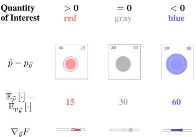
Quantity of Interest
>0 =0 <0
red gray blue
˜
p−p~θ
E˜p[·]−
Ep~θ[·]
15 30 60
[image:5.595.312.522.302.403.2]∇~θF
Figure 2: Color and area indicate differences be-twen the empirical distribution (gray outline) and model distribution. Red (or blue) indicates a model probability or parameter that should be in-creased (or dein-creased) to fit the data.
Figure 3: Gradient components use the same color coding as given in Figure 2. The length of each component indicates its potential effect on the ob-jective. Note that the sliders use a nonlinear scale from−∞to+∞.
tomatic methods come as a relief. The student may viewhintson the sliders, showing which way each slider should be nudged (Figure 3). These hints correspond to components of the log-likelihood gradient. Further automation is offered by the “Step” button, which automatically nudges all pa-rameters by taking a step of gradient ascent,12and even more by the “Solve” button, which steps all the way to the maximum.13
Our lessons guide the student to appreciate the relationship among the three activities. First, fea-ture matching is a weaker, attainable version of outcome matching (when outcome matching is
12When`
1regularization is used, the optimal~θoften con-tains many 0 weights, and a step is not permitted to jump over a (possibly optimal) weight of 0. It stops at 0, though if warranted, it can continue past 0 on the next step.
13The “Solve” button adapts the stepsize at each step, using
possible it certainly achieves feature matching as well). Second, feature matching is equivalent to maximizing the (unregularized) log-likelihood. Thus the mismatch is 0 iff the gradient of log-likelihood is 0. In fact, the mismatch equals the gradient even when they are not 0! Thus, drag-ging the sliders in the direction of the gradient hints can be viewed as a correct strategy foreither the feature matching game or the log-likelihood game. This connection shows that the current gra-dient of log-likelihood can easily be computed by summing up the observed and currently predicted counts of each feature. After understanding this and playing with the “Step” and “Solve” buttons, the student should be able to imagine writing code to train log-linear models.
5.2 Guided Exploration
We expect students to “learn by playing.” The user can experiment at any time with the sliders, with gradient ascent and its stepsize, with the type and strength of regularization, and with the size of the dataset. The user can also sample new data or new parameters, and can peek at the true parameters. These options are described further in Section 7.
We encourage experimentation by providing tooltipsthat appear whenever a student hovers the mouse pointer over a element of the GUI. Tooltips provide guidance about whatever the student is looking atright then. Some are static explanations (e.g., what does this gray bar represent?). Others dynamically update with changes to the parame-ters (e.g., the tooltips on the feature sliders show the observed and expected counts of that feature). Students see the tooltips repeatedly, which can help them absorb and reinforce concepts over an extended period of time. Students who like to learn by browsing and experimenting can point to various tooltips and get a sense of how the differ-ent concepts fit together. Some tooltips explicitly refer to one another, linking GUI elements such as the training objective, the regularization choices, and the gradient.
Though the user is welcome to play, we also provide some guidance. Each lesson displays in-structions that explain the current dataset, jus-tify modeling choices, introduce new functional-ity, lead the user through a few activities, and ask lesson-specific questions. The first lesson also links to a handout with a more formal textbook-style treatment. The last lesson links to further
Figure 4: Inventory of available shapes (circle/triangle/square/pentagon) and fills (solid/striped/hollow). Text and arbitrary im-ages may be used instead of shapes. Color and size are reserved to indicate how the current model’s predictions of outcome counts or feature counts compare to the empirical values—see Figure 2.
reading and exercises.
5.3 Instructor Interface: Creating and Tailoring Lessons
An instructor may optionally wish to tailor lessons to his or her students’ needs, interests, and abil-ities. Shapes provide a nice introduction to log-linear models, but eventually NLP students will want to think about NLP problems, whereas vi-sion students will want to think about vivi-sion prob-lems. Thus, we have designed the manipulative to handle text and arbitrary images, as well as the 12 shape-fill combinations shown in Figure 4.
Tailoring lessons to the students’ needs is as simple as editing a couple of text files. These must specify (1) a set of features, (2) a set of contexts,14 and (3) for each context, a set of featurized events, including counts and visual positions. This simple format allows one to describe some rather involved models. Some of the features may be “hidden” from the student, thereby allowing the student to experience model mismatch. Note that the visual positioning information is pedagogically impor-tant: aligning objects by orthogonal descriptions can make feature contrasts stand out more, e.g., circles vs. triangles or solid vs. striped.
The configuration files can turn off certain fea-tures on a per-lesson basis (without
program-14The set of contexts may be omitted when there is only
ming). This is useful for, e.g., hiding the “Solve” button in early lessons, adding new tooltips, or specializing the existing tooltips on a per-lesson basis.
However, being a manipulative rather than a tutoring system, our software does not monitor the user’s progress through a lesson and provide guidance via lesson-specific hints, warnings, ques-tions, or feedback. (The software is open-source, so others are free to extend it in this way.)
5.4 Back-End Implementation
Anyone can use our virtual manipulative sim-ply by visiting its website. There is no start-up cost. Aside from reading the data, model and in-structions from the web server, it is fully client-side. The Javascript back-end uses common and well-supported open-source libraries that provide a consistent experience across browsers.15 The manipulative relies on certain capabilities from the HTML5 standard. Not all browsers in current use support these capabilities, notably Internet Ex-plorer 9 and under. The tool works with recent versions of Firefox, Chrome and Safari.
6 Pedagogical Aims
6.1 Modeling and Estimation
When faced with a datasetDof(x, y)pairs, one often hopes to choose an appropriate model. When are log-linear models appropriate? Why does their hypothesis space include the uniform distribution? For what feature sets does it include everydistribution?
One should also understand statistical estima-tion. How do the features interact? When esti-mating their weights, can raising one weight alter or reverse the desired changes to other weights? How can parameter estimation go wrong statis-tically (overfitting, perhaps driving parameters to ±∞)? What might happen if we have a very large feature set? Can we design regularized es-timators that prevent overfitting (the bias-variance tradeoff)? What is the effect of the regularization constant on small and large datasets? On rare and frequent contexts? On rare and frequent features? On useful features (including features that always or never fire) and useless ones?
15Specifically and in order,d3(d3js.org/),jQuery
(jquery.com/), jQuery UI (jqueryui.com), jQuery Tools (jquerytools.org/), and qTip (craigsworks.com/projects/qtip/).
Finally, one is responsible for feature design. Which features usefully distinguish among the events? How do non-binary features work and when are they appropriate? When can a feature safely be omitted because it provides no additional modeling power? How does the choice of features affect generalization, particularly if the objective is regularized? In particular, how do shared fea-tures and backoff feafea-tures allow a model to gen-eralize to novel contexts and outcomes (or rare ones)? How do the resulting patterns of general-ization relate qualitatively to traditional smoothing techniques in NLP (Chen and Goodman, 1996)?
6.2 Training Algorithm
We also aim to convey intuitions about a specific training algorithm. We use the regularized condi-tional log-likelihood (2) to define the goodness of a parameter vector~θ. The best choice is then the~θ
that solves equation (4):
0 =∇~θF =Ep˜
h ~
f(X, Y)i−Ep~
θ
h ~
f(X, Y)i
−C∇~θR(~θ)
(4) where because our model is conditional,p~θ(x, y) denotes the hybrid distributionp˜(x)·pθ~(y|x).
Many important concepts are visible in (2) and (4). As discussed earlier, (4) includes the dif-ference between observed and expected feature counts,
Ep˜
h ~
f(X, Y)i−Ep~
θ
h ~
f(X, Y)i. (5)
Students must internalize this concept and the meaning of the two counts above. This prepares them to understand the extension to structured pre-diction, where these counts can be more diffi-cult to compute (see Section 8). It also prepares them to generalize to training latent-variable mod-els (Petrov and Klein, 2008). In that setting, the observed count can no longer be observed but is replaced by another expectation under the model, conditioned on the partial training data.
(4) also includes aweight decayterm for regu-larization. We allow both`1and`2regularization:
more important for small datasets, since for larger datasets it is dominated by the log-likelihood.
Once one can compute the gradient, one can “follow” it along the surface, in a way that is guar-anteed to increase the convex objective function up to its global maximum. The “Solve” button does this and indeed one can watch the log-likelihood bar continually increase. Yet one should observe what might go wrong here as well. Gradient ascent can oscillate if a fixedstepsize is used (by click-ing “Step” repeatedly). One may also notice that “Solve” is somewhat slow to converge on some problems, which motivates considering alternative optimization algorithms (Malouf, 2002).
We should note that we are not concerned with efficiency issues, e.g., tractably computing the normalizers Z(x). Efficient normalization is a crucial practical ingredient in using log-linear models, but our primary concern is to impart a near-physical intuitive understanding of the mod-els themselves. See Section 8 or Smith (2011) for strategies on computing the normalizer.
7 Provided Lessons
In this section we provide an overview of the 18 currently available lessons. (Of course, you can work through the lessons yourself for further de-tails.) “Core” lessons that build intuition precede the “applied” lessons focused on NLP tasks or problems. Instructors should feel especially free to replace or reorder the “applied” lessons.
Core lessons1–5provide a basicintroduction
to log-linear modeling, using unconditioned distri-butions over only four shapes as shown in Figure 1. We begin by matching outcomes using just “cir-cle” and “solid” features. We discover in lesson2
that it is redundant to add “triangle” and “striped” features. In lesson3we encounter a dataset which these features cannot fit, because the shape and fill attributes are not statistically independent. We remedy this in lesson4with a conjunctive “striped triangle” feature.
Because outcome matching fails in lesson 3, lessons 3–4 introduce feature matching and log-likelihood as suitable alternatives. Lesson5briefly illustrates a non-binary feature function, “number of sides” (taking values 3, 4, and 5 on triangles, squares, and pentagons). This clarifies the match-ing of feature counts: here we are trymatch-ing to predict the total number of sides in the dataset.
Lessons6–8focus onoptimization. They move
up to the harder setting of 9 shapes with 6 fea-tures, so we tell students how to turn on the gra-dient “hints” on the sliders. We explain how these hints relate to feature matching and log-likelihood. We invite the students to try using the hints on earlier lessons—and on new random datasets that they can generate by clicking. In Lesson 7, we introduce the “Step” and “Solve” buttons to help even more with a difficult dataset. Students use all these GUI elements to climb the convex objective and increase the log-likelihood bar.
At this point we introduceregularization. Les-son 6 invited students to generate small random datasets and observe their high variance and the tendency to overfit them. Lesson8 gives a more dramatic illustration of overfitting: with no ob-served pentagons, the solver sends θpentagon →
−∞to makep~θ(pentagon) → 0. We prevent this by adding a regularization penalty, which reserves some probability for pentagons. Striped pentagons turn out to be the least likely pentagons, because stripes were observed to be uncommon on other shapes (so θstriped < 0). Thus we see that our
choice of features allows this “smoothing method” to make useful generalizations about novel out-comes.
Lessons 9–10 consider the effect of `1 versus
`2regularization, and the competition between the regularizer (scaled by the constantC) and the log-likelihood (scaled by the dataset sizeN).16
Lessons 11–13 introduce conditional models, showing how features are shared among three con-texts. The third context is unobserved, yet our trained model makes plausible predictions about it. The conditional probabilities of unobserved shapes are positive even without regularization, in contrast to thejointprobabilities in lesson9.
We see that a frequent context xgenerally has more influence on the parameters. But this need not be true if the parameters do not help to distin-guish among the particular outcomesY(x).
Lessons14–15explore feature design in condi-tional models. We model condicondi-tional probabilities of the form p(fill | shape). “Unigram” features can favor certain fills y regardless of the shape. “Bigram” features that look at y and x together can favor different fills for each shape type. We see that features that dependonly on the shapex
cannot distinguish among fills y, and so have no
16Clever students may think to try settingC < 0, which
effect on the conditional probabilitiesp(y|x). Lesson 15 illustrates how regularization pro-motes generalization and feature selection. Once we have a full set of bigram features, the uni-gram features are redundant. We never have to put a high weight on “solid”: we can accomplish the same thing by putting high weights on “solid triangle” and “solid circle” separately. Yet this misses a generalization because it does not pre-dict that “solid” is also likely for pentagons. For-tunately, regularization encourages us to avoid too many high weights. So we prefer to put a single high weight on “solid,” and use the “solid triangle” and “solid circle” features only to model smaller shape-specific deviations from that generalization. As a result, we will indeed extrapolate that pen-tagons tend to be solid as well.
Lesson 16 begins the application-driven lessons:
One lesson builds on the “unigram” and “bi-gram” concepts to create a “bigram language model”—a model of shape sequences over a vo-cabulary of 9 shapes. A shape’s probability de-pends not only on its attributes but also on the attributes that it shares with the previous shape. What is the probability of a striped square given that the previous shape was also striped, or a square, or a striped square?
We also apply log-linear modeling to the task of text categorization (spam detection). We chal-lenge the students to puzzle out how this model is set up and how to generalize it to three-way categorization. Our contexts in this case are documents—actually very short phrases. Most contexts are seen only once, with an outcome of ei-ther “mail” or “spam.” Our feature set implements logistic regression (footnote 1): each feature con-joins y = spam with some property of the text
x, such as “contains ’parents’,” “has boldface,” or “mentions money.”
Additional linguistic application lessons may be added in the near future—e.g., modeling the rela-tive probability of grammar rules or parse trees.
The final lesson summarizes what has been learned, mentions connections to other ideas in machine learning, and points the student to further resources.
8 Graduating to Real Applications
At the time of writing, 3266 papers in the ACL Anthology mention log-linear models, with 137
using “log-linear,” “maximum entropy” or “max-ent” in the paper title. These cover a wide range of applications that can be considered in lectures or homework projects.
Early papers may cover the most fundamen-tal applications and the clearest motivation. Con-ditional log-linear models were first popularized in computational linguistics by a group of re-searchers associated with the IBM speech and lan-guage group, who called them “maximum entropy models,” after a principle that can be used to mo-tivate their form (Jaynes, 1957). They applied the method to various binary or multiclass classifica-tion problems in NLP, such as preposiclassifica-tional phrase attachment (Ratnaparkhi et al., 1994), text catego-rization (Nigam et al., 1999), and boundary pre-diction (Beeferman et al., 1999).
Log-linear models can be also used for struc-tured prediction problems in NLP such as tagging, parsing, chunking, segmentation, and language modeling. A simple strategy is to reduce struc-tured prediction to a sequence of multiclass pre-dictions, which can be individually made with a conditional log-linear model (Ratnaparkhi, 1998). A more fully probabilistic approach—used in the original “maximum entropy” papers—is to use (1) to define the conditional probabilities of the steps in a generative process that gradually produces the structure (Rosenfeld, 1994; Berger et al., 1996).17 This idea remains popular today and can be used to embed rich distributions into a variety of gener-ative models (Berg-Kirkpatrick et al., 2010). For example, a PCFG that uses richly annotated non-terminals involves a large number of context-free rules. Rather than estimating their probabilities separately, or with traditional backoff smoothing, a better approach is to use (1) to model the proba-bility of all rules given their left-hand sides, based on features that consider attributes of the nonter-minals.18
The most direct approach to structured predic-tion is to simply predict the structured output all at once, so thatyis a large structured object with many features. This is conceptually natural but means that the normalizer Z(x) involves sum-ming over a large space Y(x) (footnote 3). One
17Even predicting the single next word in a sentence can be
broken down into a sequence of binary decisions in this way. This avoids normalizing over the large vocabulary (Mnih and Hinton, 2008).
18E.g., case, number, gender, tense, aspect, mood, lexical
can restrict Y(x) before training (Johnson et al., 1999). More common is to sum efficiently by dynamic programming or sampling, as is typical in linear-chain conditional random fields (Lafferty et al., 2001), whole-sentence language modeling (Rosenfeld et al., 2001), and CRF CFGs (Finkel et al., 2008). This topic is properly deferred until such algorithmic techniques are introduced later in an NLP class, for example in a unit on parsing (see discussion in section 2). We prepare students for it by mentioning this point in our final lesson.19
Our final lesson also leads to a web page where we link to log-linear software and to various pencil-and-paper problems, homework projects, and readings that an instructor may consider as-signing. We welcome suggested additions to this page.
9 Conclusion
We have introduced an open-source, web-based virtual manipulative for log-linear models. In-cluded with the code are 18 lessons peppered with questions, a handout that gives a formal treatment of the necessary derivations, and auxiliary infor-mation including further reading, practice prob-lems, and recommended software. A version is available at http://cs.jhu.edu/˜jason/ tutorials/loglin/.
Acknowledgements We would like to thank the anonymous reviewers for their helpful feedback and suggestions and the entire Fall 2012 Natural Language Processing course at Johns Hopkins.
References
Doug Beeferman, Adam Berger, and John Lafferty. 1999. Statistical models for text segmentation. Ma-chine Learning, 34(1–3):177–210.
Taylor Berg-Kirkpatrick, Alexandre Bouchard-Cˆot´e, DeNero, John DeNero, and Dan Klein. 2010. Pain-less unsupervised learning with features. In Pro-ceedings of NAACL, June.
Adam L. Berger, Stephen A. Della Pietra, and Vin-cent J. Della Pietra. 1996. A maximum-entropy approach to natural language processing. Compu-tational Linguistics, 22(1):39–71.
19
This material can also be connected to other topics in machine learning. Dynamic programming and sampling are also used for exact or approximate computation of normal-izers in undirected graphical models (Markov random fields or conditional random fields), which are really just log-linear models for structured prediction of tuples.
Steven Bird, Ewan Klein, and Edward Loper. 2009. Natural Language Processing with Python. O’Reilly Media.
Kira J. Carbonneau, Scott C. Marley, and James P. Selig. 2013. A meta-analysis of the efficacy of teaching mathematics with concrete manipulatives.
Journal of Educational Psychology, 105(2):380 – 400.
Stanley Chen and Joshua Goodman. 1996. An empir-ical study of smoothing techniques. InProceedings of ACL.
Douglas H. Clements and Sue McMillen. 1996. Re-thinking “concrete” manipulatives. Teaching Chil-dren Mathematics, 2(5):pp. 270–279.
Hal Daum´e III. 2004. Notes on CG and LM-BFGS optimization of logistic regression. Paper available at http://pub.hal3.name# daume04cg-bfgs, implementation available at
http://hal3.name/megam/, August.
Jason Eisner. 2002. An interactive spreadsheet for teaching the forward-backward algorithm. In Dragomir Radev and Chris Brew, editors, Proceed-ings of the ACL Workshop on Effective Tools and Methodologies for Teaching NLP and CL, pages 10– 18, Philadelphia, July.
Jenny Rose Finkel, Alex Kleeman, and Christopher D Manning. 2008. Efficient, feature-based, condi-tional random field parsing. Proceedings of ACL-08: HLT, pages 959–967.
E. T. Jaynes. 1957. Information theory and statistical mechanics.Physics Reviews, 106:620–630.
Mark Johnson, Stuart Geman, Stephen Canon, Zhiyi Chi, and Stefan Riezler. 1999. Estimators for stochastic “unification-based” grammars. In Pro-ceedings of ACL.
John Lafferty, Andrew McCallum, and Fernando Pereira. 2001. Conditional random fields: Prob-abilistic models for segmenting and labeling se-quence data. InProceedings of ICML.
Marc Light, Robert Arens, and Xin Lu. 2005. Web-based interfaces for natural language processing tools. InProceedings of the Second ACL Workshop on Effective Tools and Methodologies for Teaching NLP and CL, pages 28–31, Ann Arbor, Michigan, June. Association for Computational Linguistics.
Adam Lopez, Matt Post, Chris Callison-Burch, Jonathan Weese, Juri Ganitkevitch, Narges Ah-midi, Olivia Buzek, Leah Hanson, Beenish Jamil, Matthias Lee, et al. 2013. Learning to translate with products of novices: Teaching MT with competi-tive challenge problems. Transactions of the ACL (TACL), 1.
Andriy Mnih and Geoffrey Hinton. 2008. A scalable hierarchical distributed language model. In Pro-ceedings of NIPS.
Patricia S. Moyer, Johnna J. Bolyard, and Mark A. Spikell. 2002. What are virtual manipulatives?
Teaching Children Mathematics, 8(6):372–377.
Kamal Nigam, John Lafferty, and Andrew McCallum. 1999. Using maximum entropy for text classifica-tion. In IJCAI-99 Workshop on Machine Learning for Information Filtering, pages 61–67.
Jan Nouza, Miroslav Holada, and Daniel Hajek. 1997. An educational and experimental workbench for vi-sual processing of speech data. InFifth European Conference on Speech Communication and Technol-ogy.
Slav Petrov and Dan Klein. 2008. Sparse multi-scale grammars for discriminative latent variable parsing. InProceedings of EMNLP, pages 867–876, October.
Adwait Ratnaparkhi, Jeff Reynar, and Salim Roukos. 1994. A maximum entropy model for prepositional phrase attachment. InProceedings of the ARPA Hu-man Language Technology Workshop, pages 250– 255.
Adwait Ratnaparkhi. 1998. Maximum Entropy Models for Natural Language Ambiguity Resolution. Ph.D. thesis, University of Pennsylvania, July.
Ronald Rosenfeld, Stanley F. Chen, and Xiaojin Zhu. 2001. Whole-sentence exponential language mod-els: A vehicle for linguistic-statistical integration.
Computer Speech and Language, 15(1).
Ronald Rosenfeld. 1994. Adaptive Statistical Lan-guage Modeling: A Maximum Entropy Approach. Ph.D. thesis, Carnegie Mellon University.
Noah A. Smith. 2011. Linguistic Structure Prediction. Synthesis Lectures on Human Language Technolo-gies. Morgan and Claypool, May.
Evelyn J Sowell. 1989. Effects of manipulative materi-als in mathematics instruction. Journal for Research in Mathematics Education, pages 498–505.
Michel Tokic and Haitham Bou Ammar. 2012. Teach-ing reinforcement learnTeach-ing usTeach-ing a physical robot. InProceedings of the ICML Workshop on Teaching Machine Learning.