Approximation of Finite Population Totals Using Lagrange Polynomial

(1)

ISSN Online: 2161-7198 ISSN Print: 2161-718X

DOI: 10.4236/ojs.2017.74048 Aug. 18, 2017 689 Open Journal of Statistics

Approximation of Finite Population Totals

Using Lagrange Polynomial

Lamin Kabareh

1*

, Thomas Mageto

2

, Benjamin Muema

2

1_{Pan African University Institute for Basic Sciences, Technology and Innovation (PAUSTI), Nairobi, Kenya} 2_{Jomo Kenyatta University of Agriculture and Technology, Nairobi, Kenya}

Abstract

Approximation of finite population totals in the presence of auxiliary infor-mation is considered. A polynomial based on Lagrange polynomial is pro-posed. Like the local polynomial regression, Horvitz Thompson and ratio es-timators, this approximation technique is based on annual population total in order to fit in the best approximating polynomial within a given period of time (years) in this study. This proposed technique has shown to be unbiased under a linear polynomial. The use of real data indicated that the polynomial is efficient and can approximate properly even when the data is unevenly spaced.

Keywords

Lagrange Polynomial, Approximation, Finite Population Total, Auxiliary Information, Local Polynomial Regression,

Horvitz Thompson and Ratio Estimator

1. Introduction

This study is using an approximation technique to approximate the finite popu-lation total called the Lagrange polynomial that doesn’t require any selection of bandwidth as in the case of local polynomial regression estimator. The Lagrange polynomials are used for polynomial interpolation and extrapolation. For each given set of distinct points xjand yj, the Lagrange polynomial of the lowest de-gree takes on each point xjcorresponding to yj(i.e. the functions coincide at each point). Although named after Joseph Louis Lagrange, who published it in 1795, the method was first discovered in 1779 by Edward Waring. It is also an easy consequence of a formula published in 1783 by Leonhard Euler as will be seen later on how it works.

How to cite this paper: Kabareh, L., Mage-to, T. and Muema, B. (2017) Approximation of Finite Population Totals Using Lagrange Polynomial. Open Journal of Statistics, 7, 689- 701.

https://doi.org/10.4236/ojs.2017.74048

Received: July 9, 2017 Accepted: August 15, 2017 Published: August 18, 2017

http://creativecommons.org/licenses/by/4.0/

(2)

DOI: 10.4236/ojs.2017.74048 690 Open Journal of Statistics [1] in the context of using auxiliary information from survey data to estimate the population total defined U U1, , ,2 UN as the set of labels for the finite population. Letting

(

y xi, i

)

be the respective values of the study variable y and the auxiliary variable x attached to ith_{unit. Of interest is the estimation of} popu-lation total Yt =

∑

iN=₁xi using the known population totals 1

N

t i i

X =

∑

₌ x _{at the} estimation stage, if we let s s1, , ,2 sn be the set of sampled units under a gen-eral sampling design p, and let

π

i = p i s

(

∈

)

be the first order inclusion proba-bilities. In 1940, Cochran made an important contribution to the modern sam-pling theory by suggesting methods of using the auxiliary information for the purpose of estimation in order to increase the precision of the estimates [2]. He developed the ratio estimator to estimate the population mean or the total of the study variable y. The ratio estimator of population Y is of the form

; 0

r _xyX

y = x≠

The aim of this method is to use the ratio of sample means of two characters which would be almost stable under sampling fluctuations and, thus, would pro-vide a better estimate of the true value. It has been well-known fact that yr is most efficient than the sample mean estimator y, where no auxiliary informa-tion is used, if ρyx, the coefficient of correlation between y and x, is greater than half the ratio of coefficient of variation of x to that of y, that is, if

1 2 x

yx

y C C

ρ > _ _

  (1.0)

Thus, if the information on an auxiliary variable is either already available or can be obtained at no extra cost and it has a high positive correlation with the main character, one would certainly prefer ratio estimator to develop more and more superior techniques to reduce bias and also to obtain unbiased estimators with greater precision by modifying either the sampling schemes or the estimation procedures or both. [3] further extended the work of [4] on systematic sampling. [5] also dealt with the problem of estimation using the priori-information. Con-trary to the situation of ratio estimator, if variables y and x are negatively corre-lated, then the product estimator of population mean Y is of the form

; 0

q _Xy x

y = X ≠ (1.1) that was proposed by [6]. It has been observed that the product estimator gives higher precision than the sample mean estimator y under the condition that is if

1 2 x

yx

y C C

ρ ≤ − _ _

  (1.2)

The expressions for bias and mean square errors of yr and yq have been derived by [7].

(3)

DOI: 10.4236/ojs.2017.74048 691 Open Journal of Statistics

(

)

d X

y =y+β −x

₍₁_.₃₎ where β is a constant. The best choice of β which minimizes the variance of the estimator is seen to be

2

yx

x

S S

β =

(1.4) which is the population regression coefficient of y on x. Since, β is generally un-known in practice, it is estimated by sample regression coefficient

2

yx

x

s b

s

= _(1.5)

Using sample regression coefficient (i.e. b), Watson defined simple linear re-gression estimator as

(

)

1r

y = +y b X x+ (1.6) This estimator is biased, the bias being negligible for large samples.

The most common way of defining a more efficient class of estimators than usual ratio (product) and sample mean estimator is to include one or more un-known parameters in the estimators whose optimum choice is made by mini-mizing the corresponding mean square error or variance. Sometimes, such mod-ifications or generalizations are made by mixing two or more estimators with unknown weights whose optimum values are then determined which generally depend upon population parameters. In order to propose efficient classes of es-timators, [9] suggested a one-parameter family of factor-type (F-T) ratio esti-mators defined as

(

)

(

)

f

A C fBx

y y

A fB Cx

X X

 + + 

=  ₊ ₊ 

 

  (1.7)

where A d=

(

−1

)(

d−2

)

, B=

(

d−1

)(

d−4

)

, C=

(

d−2

)(

d−3

)(

d−4

)

,

0

d> , f n N

= _{. The literature on survey sampling describes a great variety of}

techniques of using auxiliary information to obtained more efficient estimators. Keeping this fact in view, a large number of authors have paid their attention toward the formulation of modified ratio and product estimators using informa-tion on an auxiliary variate, for instance, see [10] and Singh et al. [11].

Suppose n is large and MSE R Var R

( )

ˆ =

( )

ˆ _{. We assume that} x and X are quite close such that

ˆ x x

x

y R y R

R

X

R − −

− = =

so that the bias of R becomes quite small.

(4)

DOI: 10.4236/ojs.2017.74048 692 Open Journal of Statistics following estimator for population total of the variable y. The estimator could also be written as

( )

1

ˆ

ˆ i N _ˆ i

gen j

i s i j i s i

x y

Y

µ

x

µ

π

∈ = ∈

 

= +_ − _

 

∑

(1.8)

The first term in (1.8) is a design estimator which the second is model com-ponent. Therefore, when the sample comprises of the whole population, the model component reduces to zero since πi= 1 and s = N. We therefore have the actual population total. [13] proposed the super population model ξ, such that

( )

i

( )

i

E yξ =

µ

x where

µ

( )

xi is a known function of xi. They proposed model calibration estimator for population total Ytto be _{i s} i

i y Y=

∑

_∈ _π

In local polynomial regression, a lower-order weighted least squares (WLS) regression is fit at each point of interest, x using data from some neighborhood around x. Following the notation from [14], let the (Xi, Yi) be ordered pairs such that

( )

i i i i

Y m X= +

σ

X

ε

_(1.9) where

ε

~N

( )

0,1 _, 2

( )

i X

σ is the variance of Yiat the point Xi, and Xicomes from some distribution, f. In some cases, homoscedastic variance is assumed, so we let _σ2

( )

_X ₌_σ2_{. It is typically of interest to estimate}_m₍_x_{). Using Taylor’s}

expansion:

( )

( )(

)

( ) (

)

! n n o

o o o o

m x

m x m x m x x x x x

n

′

≈ + − + + − (1.91)

We can estimate these terms using weighted least squares by solving the fol-lowing for β:

(

0

)

(

0

)

1

2 0

j

n q

i j i h i

i= Y − j= β X −x  K X −x

∑

(1.92)

In (1.92), h controls the size of the neighborhood around x0, and Kh(.) controls

the weights, where h

( )

.

K h K h ⋅      

≡ _{, and}_K_{is a kernel function. Denote the}

solu-tion to (1.92) as

β

ˆ._{Then estimated}

( )

0 !ˆ

v

V

m x =v β . [15] proposed to use non-parametric method to obtain

µ

( )

. _{. However, this estimator experiences a twin} problem of how to determine the optimal degrees of the local polynomial. A higher degree polynomial yields a smoother

µ

( )

. but worsens the boundary variance [16]. Such estimators are challenging to employ in cases of multiple covariates and when data is sparse. Another challenge is how to incorporate ca-tegorical covariates. It is therefore necessary to consider other methods to re-cover the fitted values such as splines. The term spline originally referred to a tool used by draftsmen to draw curves. According to [17], splines are piecewise regression functions we constrain to join at points called knots.

(5)

DOI: 10.4236/ojs.2017.74048 693 Open Journal of Statistics doesn’t make use of the auxiliary information xibut instead uses only the study variable yito obtain the population total.

Consider the population of size N with units y y y1, , , ,2 3 yN. Suppose we want to select sample s of size ns.

Let πi be the probability of including ithunit of the population in sample s. This is called the inclusion probability or first order inclusion probability of ith unit in the sample.

Let πijbe the probability of including ith and jth units in the sample. This is called the joint inclusion probability or second order inclusion probability.

When the sample is obtained from a probability sampling design, an unbiased estimator for the Total N₁

i i

Y=

∑

= y is given by

1

1 1

ˆ N i N

HT i i

i i i

y

Y yπ

π −

= =

=

_∑

=

_∑

_(1.93)

ˆ_HT

Y is unbiased under design based approach [19]

Variance

( )

(

)

1 1

ˆ N N i j

HT ij i j

i j i j

y y

V Y π π π

π π

= =

=

∑∑

−

The variance of this estimator can be minimized when πi∝yi. That is, if the first order inclusion probability is proportional to yi, the resulting HT estimator under this sampling design will have zero variance. However, in practice, we can’t construct such design because we don’t know the value of yi in the design stage. If there is a good auxiliary variable xiwhich is believed to be closely related with yi, then a sampling design with πi ∝xican lead to very efficient sampling design This method of estimating the finite population totals doesn’t make use of the auxiliary information xibut instead uses only the study variable yi to ob-tain the population totals.

Research literature has revealed that the ratio estimator performs better than the local linear polynomial estimator when the population is linear no matter which variance is used. The local linear polynomial regression estimator be-comes a better estimator when the population used is either quadratic or expo-nential especially with an increase in the sample size which increases the likelih-ood of outliers in the sample.

One of the most useful and well-known classes of functions mapping the set of real numbers into itself is algebraic polynomials, the set of functions of the form

( )

1

1 1 0

n n

n n n

P x a x a x − a x a

−

= + ++ +

(6)

DOI: 10.4236/ojs.2017.74048 694 Open Journal of Statistics In Section 2 we briefly introduced the Lagrange polynomial and in Section 2.1 we further defined the Lagrange polynomial. Section 2.2 talked about properties of polynomial approximations and proof of the Karl Weierstrass theorem. Sec-tion 3 talked about the main results with the use of real data from the Kenya Na-tional Bureau of Statistics on population census. While Section 3.2 showed how to calculate missing values via interpolation. Section 3.3 and 3.4 extrapolated the population totals in 2009 and 2019 respectively. Section 4 concluded by stating that, the best approximating polynomial for a quick convergence must be a li-near one in order to give a better extrapolation.

2. Approximation of Finite Population Totals

In this section, we are basically introducing an approximator that is the La-grange polynomial approximate of the finite population totals.

2.1. Proposed Lagrange Polynomial

Consider a finite population U=

{

U U1, , ,2UN

}

of N units. Let (y, x) be the (total, year) variables taking non negative real values (yi, xi) respectively, on the unit U ii

(

=1,2, , N

)

. From the population U, a simple random sample of size

n is drawn without replacement. Then, the Lagrange interpolating polynomial is the polynomial p(x) of degree ≤ (n − 1) that passes through the n points

( )

(

x y1, 1= f x1

)

,

(

x y2, 2= f x

( )

2

)

, ,

(

x yn, n= f x

( )

n

)

and is given by:

( )

n₁

( )

j j

P x =

∑

₌ P x , where

( )

1

n k

j j k

j k

x x P x y

x x

= −

−

=

∏

_{written explicitly,}

( ) (

₍

₎₍

)(

) (

_{) (}

)

₎

₍

(

₎₍

)(

) (

_{) (}

)

₎

(

) (

)

(

) (

)

2 3 1 3

1 2

1 2 1 3 1 2 1 2 3 2

1 1 1 1 n n n n n n

n n n

x x x x x x x x x x x x

P x y y

x x x x x x x x x x x x

x x x x

y

x x x x

− − − − − − − − = + − − − − − − − − + + − −

2.2. Asymptotic Properties of Polynomial Approximations

Polynomial Approximation of Functions: Weierstrass Theorem:

[ ]

: ,

f a b →R continuous

Then there exists a sequence of polynomials Pn(x) such that

[ ],

( )

max 0

n x a b n

f P− ∞= ∈ f x −P x → as n → ∞ Proof of Theorem:

[ ] [ ]

: , 0,1

f a b = →R continuous.

( )

( )( )

₍

₎

(

)

0

! ₁

!

n _{n k}

k

n n

k

n k

P x B f x f x x

k n k n

(7)

0 as

n

f P− _∞→ n→ ∞

We are going to consider three functions: f x

( )

=1_, f x

( )

=x _and _{f x}

( )

₌_x2

and show convergence.

( )

1

f x =

( )( )

₍

_{) (}

)

(

)

0

! ₁ ₁ _1, ₀

! !

n _{n k} _n

k n

k

n

B f x x k x x n

k n k

− = = − = + − = ≥ −

∑

Hence

( )

0

n f B f− _∞ =

Also,

( )

f x =x

( )( )

₍

₎

(

)

(

)

(

) (

)

0 1 ! ₁ ! ! 1 ! 1

1 ! !

n _{n k}

k n

k

n _{n k}

k

n k

B f x x k

k n k n n

x x

k n k

− = − = = − − − = − − −

∑

Let L k= −1

(

)

(

) (

)

1 1 0 1 ! 1

! 1 !

n _n _L

L

n

x x x

L n L

− − − = − = − − −

∑

Hence

( )

0, 1

n

B f − f _∞ = n≥

( )

2

f x =x

(

)

(

) (

)

(

)

(

)

(

) (

)

(

)

(

) (

)

) (

)

1 2 1

1 ! 1 1 ₁ 1 ! !

1 ! 1 ₁ 1 1 ! ₁

2 ! ! 1 ! !

n

n k k

k

n _{n k} n _{n k}

k k

n k _x _x

k n k n

n n

x x x x

k n k n n k n k

− = − − = = − − + = − − − − − = − + − − − − −

∑

( )( ) (

)

2

₍

(

_{) (}

)

₎

2

(

)

2

1 2 ! ₁ 1

2 ! !

n _{n k}

k n

k

n n

B f x x x x x

n k n k n

− − = − − = − + − −

∑

( )

1 0 as 4

n

f B f n

n ∞

− = → → ∞

In order to obtain a best approximating polynomial that has less error, one needs to choose a linear interpolating points that is closest to the target point

3. Main Results

3.1. Data Exploration

(8)

[image:8.595.209.536.66.318.2]

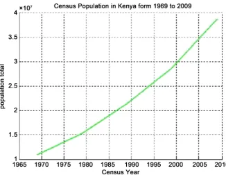
Figure 1. The Kenya population census data since 1969 to 2009 were plotted to see the behaviour of the data as soon shown above in green.

However, we aimed at selecting a sample size of two from 1969 to 2009 popu-lation census using a technique of simple random sampling without replacement making a sample total of ten. A pair of linear samples selected were plotted on the same charts to approximate the function f(x) in green colour as shown below for each.

The chart in (Figure 2) below comprises of two linear polynomials that have uniformly approximated the function in green in order to give a better approx-imate to the population total in 2019. As can be seen, the two linear plots are not showing any better approximate of the function f(x) in green in order to help us extrapolate the population total in 2019.

The linear polynomials in (Figure 3) below in red and blue are used to un-iformly approximate the function f(x) in green so as to help us extrapolate the population total in 2019. This was clearly seen to have obtained high variation in the approximation. The blue line appeared to be better than the red at the end point.

Similarly, the approximating linear polynomials in red and green in (Figure 4) are used to approximate the function f(x) in green. Unfortunately, the two approximating lines are not suitable to help extrapolate the population total in 2019.

The approximating linear polynomials shown below in (Figure 5) are used to uniformly approximate the function f(x) in green representing the trend of the entire population. As seen on the chart, the black line appeared to perform bet-ter at the end point than the blue but showed some variations.

(9)

[image:9.595.210.534.113.375.2]

un-DOI: 10.4236/ojs.2017.74048 697 Open Journal of Statistics iformly approximate the function f(x) representing the total population trend per year. The chart has clearly shown that, the black dotted line depicted the best

Figure 2. This chart was obtained from a set of data ranging from [1969, 1979] in yellow to [1969, 1989] in blue and the green function (f(x)).

[image:9.595.208.537.417.694.2]

(10)

[image:10.595.209.537.85.350.2]

Figure 4. This chart was obtained from a set of data ranging from [1979, 1989] in green dotted line to [1979, 1999] in red and the green function(f(x)).

[image:10.595.208.536.404.667.2]

(11)

[image:11.595.209.537.67.329.2]

Figure 6. This chart was obtained from a set of data ranging from [1989, 2009] in red dotted line to [1999, 2009] in black dotted line and the green function (f(x)).

approximate on its entire interval which is [1999, 2009] as the place for the Best Approximating Polynomial (BAP) to approximate the function f(x) uniformly to any degree of accuracy.

3.2. Calculating Missing Values via Interpolation

[ ] [

1 1999

]

x = and y

[ ] [

1 = 28,686,607

]

; x

[ ] [

11 = 2009

]

and

[ ] [

11 38,610,097

]

y =

Columns 1 through 8

28,686,607 29,678,956 30,671,305 31,663,654 32,656,003 33,648,352 34,640,701 35,633,050

Columns 9 through 11

36,625,399 37,617,748 38,610,097

[ ] [ ]

1

(

[ ] [ ]

11 1

)

y i =y i− + y −y i− h where i ≥ 2 and h = annual step size

3.3. Approximation of Population Total in 2009

[ ] [

11 2009

]

x = _and y

[ ] [

11 = 38,610,097

]

_given

[ ] [

10 2008

]

x = and y

[ ] [

10 = 37,617,748

]

approximated

[ ] [

9 2007

]

x = _and y

[ ] [

9 = 36,625,399

]

_approximated

[ ] [ ]

(

)

(

[ ] [ ]

)

[ ]

9 11 10 9 10 9

L = x −x x −x ∗y

[ ] [ ]

(

)

(

[ ] [ ]

)

[ ]

10 11 10 10 9 10

(12)

DOI: 10.4236/ojs.2017.74048 700 Open Journal of Statistics Approximated value = L9 + L10

Approximated population total = 38,610,097 Error = 0

3.4. Extrapolation of 2019 Population Total

[ ] [

11 2009

]

x = _and y

[ ] [

11 = 38,610,097

]

[ ] [

10 2008

]

x = and y

[ ] [

10 = 37,617,748

]

[ ]

(

)

(

[ ] [ ]

)

[ ]

19 2019 11 10 11 10

L = −x x −x ∗y

[ ]

(

)

(

[ ] [ ]

)

[ ]

20 2019 10 11 10 11

L = −x x −x ∗y

Approximated value = L19 + L20

Approximated population total = 48,533,587

4. Conclusion

In this work, the Lagrange polynomial has proven to be a good technique in ap-proximating the population total from data obtained from the Kenya National Bureau of Statistics (KNBS). The research revealed that, subsequent population totals can better be approximated using a sample closest to the target population being approximated. Therefore, the best approximating polynomial must be a linear form in order to obtain convergence with a diminishing variation in a given interval. The precision of this technique can better be measured with the outcome obtained in the interpolation of missing values shown in the results above to extrapolate the population total in 2009 which was equal to the exact population obtained in that census. We therefore conclude that, the population of Kenya for the 2019 census will be forty-eight million five hundred and thir-ty-three thousand five hundred and eighty-seven.

Acknowledgements

We are grateful to the authors for their numerous and valuable contributions to this work, most especially the first author.

Conflict of Interest

The author(s) declare(s) that there is no conflict of interest regarding the publi-cation of this paper.

References

[1] Deville, J.-C. and Sarndal, C.-E. (1992) Calibration Estimators in Survey Sampling. Journal of the American Statistical Association, 87, 376.

https://doi.org/10.1080/01621459.1992.10475217

[2] Cochran, W.G. and Goulden, C.H. (1940) Methods of Statistical Analysis. Journal of the Royal Statistical Society, 103, 250. https://doi.org/10.2307/2980420

(13)

DOI: 10.4236/ojs.2017.74048 701 Open Journal of Statistics [4] Nadaraya, E.A. (1964) On Estimating Regression. Theory of Probability and Its

Ap-plications, 9, 141-142. https://doi.org/10.1137/1109020

[5] Singh, V.K., Singh, H.P., Singh, H.P. and Shukla, D. (1994) A General Class of Chain Estimators for Ratio and Product of Two Means of a Finite Population. Communications in Statistics Theory and Methods, 23, 1341-1355.

https://doi.org/10.1080/03610929408831325

[6] Searls, D.T. (1964) The Utilization of a Known Coefficient of Variation in the Esti-mation Procedure. Journal of the American Statistical Association, 59, 1225. https://doi.org/10.1080/01621459.1964.10480765

[7] Wu, C. and Sitter, R.R. (2001) A Model-Calibration Approach to Using Complete Auxiliary Information from Survey Data. Journal of the American Statistical Asso-ciation, 96, 185-193. https://doi.org/10.1198/016214501750333054

[8] Johnson, A.A., Breidt, F.J. and Opsomer, J.D. (2008) Estimating Distribution Func-tions from Survey Data Using Nonparametric Regression. Journal of Statistical Theory and Practice, 2, 419-431. https://doi.org/10.1080/15598608.2008.10411884 [9] Sukhatme, V. (1984) Future Dimensions of World Food and Population. Economic

Development and Cultural Change, 32, 892-897. https://doi.org/10.1086/451435 [10] Watson, G. (1964) Smooth Regression Analysis. The Indian Journal of statistics

Se-ries A, 26, 359-372.

[11] Solanki, R.S., Singh, H.P. and Pal, S.K. (2014) Improved Ratio-Type Estimators of Finite Population Variance Using Quartiles. Hacettepe Journal of Mathematics and Statistics, 45, 1. https://doi.org/10.15672/HJMS.2014448247

[12] Lairez, P. (2016) A Deterministic Algorithm to Compute Approximate Roots of Po-lynomial Systems in PoPo-lynomial Average Time. Foundations of Computational Mathematics. https://doi.org/10.1007/s10208-016-9319-7

[13] Godambe, V.P. and Thompson, M.E. (1986) Parameters of Super Population and Survey Population: Their Relationships and Estimation. International Statistical Re-view/Revue International de Statistique, JSTOR, 127-138.

[14] Hansen, M.H., Hurwitz, W.N. and Madow, W.G. (1953) Sample Survey Methods and Theory. Vol. 1, Wiley, New York.

[15] Robson, D.S. (1957) Applications of Multivariate Polykays to the Theory of Un-biased Ratiotype Estimation. Journal of the American Statistical Association, 52, 511-522. https://doi.org/10.1080/01621459.1957.10501407

[16] Montanari, G.E. and Ranalli, M.G. (2003) On Calibration Methods for Design Based Finite Population Inferences. Bulletin of the International Statistical Institute, 54th Session 60.

[17] Madow, W.G. and Madow, L.H. (1944) On the Theory of Systematic Sampling, I. The Annals of Mathematical Statistics, 15, 1-24.

https://doi.org/10.1214/aoms/1177731312

[18] Keele, L.J. (2008) Semiparametric Regression for the Social Sciences. John Wiley and Sons.

[19] Singh, H.P., Pal, S.K. and Mehta, V. (2016) A Generalized Class of Ratio-Cum-Dual to Ratio Estimators of Finite Population Mean Using Auxiliary Information in Sample Surveys. Mathematical Sciences Letters, 5, 203-211.

https://doi.org/10.18576/msl/050215

(14)

Submit or recommend next manuscript to SCIRP and we will provide best service for you:

Accepting pre-submission inquiries through Email, Facebook, LinkedIn, Twitter, etc. A wide selection of journals (inclusive of 9 subjects, more than 200 journals)

Providing 24-hour high-quality service User-friendly online submission system Fair and swift peer-review system

Efficient typesetting and proofreading procedure

Display of the result of downloads and visits, as well as the number of cited articles Maximum dissemination of your research work