Graph based Learning for Statistical Machine Translation

Graph-based Learning for Statistical Machine Translation

Andrei Alexandrescu

Dept. of Comp. Sci. Eng. University of Washington Seattle, WA 98195, USA

[email protected]

Katrin Kirchhoff

Dept. of Electrical Eng. University of Washington

Seattle, WA 98195, USA

[email protected]

Abstract

Current phrase-based statistical machine translation systems process each test sentence in isolation and do not enforce global consis-tency constraints, even though the test data is often internally consistent with respect to topic or style. We propose a new consistency model for machine translation in the form of a graph-based semi-supervised learning algorithm that exploits similarities between training and test data and also similarities between different test sentences. The algo-rithm learns a regression function jointly over training and test data and uses the resulting scores to rerank translation hypotheses. Eval-uation on two travel expression translation tasks demonstrates improvements of up to 2.6 BLEU points absolute and 2.8% in PER.

1 Introduction

Current phrase-based statistical machine translation (SMT) systems commonly operate at the sentence level—each sentence is translated in isolation, even when the test data consists of internally coherent paragraphs or stories, such as news articles. For each sentence, SMT systems choose the translation hypothesis that maximizes a combined log-linear model score, which is computed independently of all other sentences, using globally optimized com-bination weights. Thus, similar input strings may be translated in very different ways, depending on which component model happens to dominate the combined score for that sentence. This is illustrated by the following example (from the IWSLT 2007

Arabic-English translation task):

Source 1: Asf lA ymknk *lk hnAk klfp HwAly vmAnyn dwlAr lAlsAEp AlwAHdp

Ref: sorry you can’t there is a cost the charge is eighty dollars per hour

1-best: i’m sorry you can’t there in the cost about eighty dollars for a one o’clock

Source 2: E*rA lA ymknk t$gyl AltlfAz HtY tqlE AlTA_}rp

Ref: sorry you cannot turn the tv on until the plane has taken off

1-best: excuse me i you turn tv until the plane departs

The phrase lA ymknk (you may not/you cannot) is translated differently (and wrongly in the sec-ond case) due to different segmentations and phrase translations chosen by the decoder. Though differ-ent choices may be sometimes appropriate, the lack of constraints enforcing translation consistency of-ten leads to suboptimal translation performance. It would be desirable to counter this effect by encour-aging similar outputs for similar inputs (under a suit-ably defined notion of similarity, which may include e.g. a context specification for the phrase/sentence).

In machine learning, the idea of forcing the out-puts of a statistical learner to vary smoothly with the underlying structure of the inputs has been formal-ized in the graph-based learning (GBL) framework. In GBL, both labeled (train) and unlabeled (test) data samples are jointly represented as vertices in a graph whose edges encode pairwise similarities be-tween samples. Various learning algorithms can be applied to assign labels to the test samples while en-suring that the classification output varies smoothly

along the manifold defined by the graph. GBL has been successfully applied to a range of problems in computer vision, computational biology, and natu-ral language processing. However, in most cases, the learning tasks consisted of unstructured classi-fication, where the input was represented by fixed-length feature vectors and the output was one of a finite set of discrete labels. In machine translation, by contrast, both inputs and outputs consist of word strings of variable length, and the number of possi-ble outputs is not fixed and practically unlimited.

In this paper we propose a new graph-based learn-ing algorithm with structured inputs and outputs to improve consistency in phrase-based statistical ma-chine translation. We define a joint similarity graph over training and test data and use an iterative label propagation procedure to regress a scoring function over the graph. The resulting scores for unlabeled samples (translation hypotheses) are then combined with standard model scores in a log-linear transla-tion model for the purpose of reranking. Our con-tributions are twofold. First, from a machine trans-lation perspective, we design and evaluate a global consistency model enforcing that similar inputs re-ceive similar translations. Second, from a machine learning perspective, we apply graph-based learning to a task with structured inputs and outputs, which is a novel contribution in itself since previous ap-plications of GBL have focused on predicting cat-egorical labels. We evaluate our approach on two machine translation tasks, the IWSLT 2007 Italian-to-English and Arabic-Italian-to-English tasks, and demon-strate significant improvements over the baseline.

2 Graph-Based Learning

GBL algorithms rely on a similarity graph consisting of a set of nodes representing data samplesxi(where

iranges over1, . . . , llabeled points andl+ 1, . . . , n

unlabeled points), and a set of weighted edges en-coding pairwise similarities between samples. The graph is characterized by a weight matrixW whose elementsWij ≥0are the similarity values for edges between vertices xi and xj, and by its label vector

Y = (y1, . . . yl), yi ∈ {1, . . . , C} that defines la-bels for the firstlpoints. If there is no edge linking nodesxi and xj, thenWij = 0. There is consider-able freedom in choosing the weights. The

similar-ity measure used to compute the edge weights de-termines the graph structure and is the most impor-tant factor in successfully applying GBL. In most applications of GBL, data samples are represented by fixed-length feature vectors, and cosine similar-ity or Euclidean distance-based measures are used for edge weights.

Learning algorithms on similarity graphs include e.g. min-cut (Blum and Chawla, 2001), spectral graph transducer (Joachims, 2003), random walk-based approaches (Szummer and Jaakkola, 2001), and label propagation (Zhu and Ghahramani, 2002). The algorithm proposed herein is based on the latter.

2.1 Label Propagation

Given a graph defined by a weight matrix W and a label setY, the basic label propagation algorithm proceeds as follows:

1. Initialize the matrixPasPij = PWij−Wii

jWij−Wii

2. Initialize an_×Cmatrixf with binary vectors encoding the known labels for the first lrows:

fi =δC(yi)∀i∈ {1,2, . . . , l}, whereδC(yi)is the Kronecker vector of lengthCwith 1 in po-sitionyi and 0 elsewhere. The remaining rows off can be zero.

3. f′ _←P_×f

4. Clamp already-labeled data rows:f_i′ =δC(yi)

∀i_{∈ {}1,2, . . . , l_}

5. Iff′ ∼=f, stop. 6. f ←f′

7. Repeat from step 3.

After convergence, f contains the solution in rows

l+ 1tonin the form of unnormalized label proba-bility distributions. Hard labels can be obtained by

ˆ

yi = arg max j∈{1,...,C}

fij ∀i∈ {l+ 1, . . . , n} (1)

The algorithm minimizes the following cost func-tion (Zhu, 2005):

S=

C X

k=1 X

i>l∨j>l

Wij(fik−fjk)2 (2)

that, to the extent possible, assigns similar soft labels (identical hard labels) to nodes linked by edges with large weights (i.e., highly similar samples). The labeling decision takes into account not only sim-ilarities between labeled and unlabeled nodes (as in nearest-neighbor approaches) but also similarities among unlabeled nodes. Label propagation has been used successfully for various classification tasks, e.g. image classification and handwriting recogni-tion (Zhu, 2005). In natural language processing, la-bel propagation has been used for document classifi-cation (Zhu, 2005), word sense disambiguation (Niu et al., 2005; Alexandrescu and Kirchhoff, 2007), and sentiment categorization (Goldberg and Zhu, 2006).

3 Graph-Based Learning for Machine Translation

Our goal is to exploit graph-based learning for im-proving consistency in statistical phrase-based ma-chine translation. Intuitively, a set of similar source sentences should receive similar target-language translations. This means that similarities between training and test sentences should be taken into ac-count, but also similarities between different test

sentences, which is a source of information currently

not exploited by standard SMT systems. To this end we define a graph over the training and test sets with edges between test and training sentences as well as between different test sentences. In cases where a test sentence does not have any connections to training sentences but is connected to other test sentences, helpful information about preferred trans-lations can be propagated via these edges.

As mentioned above, the problem of machine translation does not neatly fit into the standard GBL framework. Given that our samples consist of variable-length word strings instead of feature vectors, the standard cosine or Euclidean-distance based similarity measures cannot be used mean-ingfully, and the number of possible “labels”— correct translations—is unbounded and practically very large. We thus need to modify both the graph construction and the label propagation algorithms.

First, we handle the problem of unlimited out-puts by applying GBL to rescoring only. In most SMT systems, anN-best list (generated by a first de-coding pass) approximates the search space of good

hypotheses reasonably well, provided N is large enough. For all hypotheses of all sentences in the test set (set we denote withH), the system learns a ranking functionr :H _→[0,1]. Larger values ofr

indicate better hypotheses. The corresponding loss functional is

L(r) =X

i,j

Wij[r(xi)−r(xj)]2 (3)

L(r) measures the smoothness of r over the graph by penalizing highly similar clusters of nodes that have a high variance of r (in other words, simi-lar input sentences that have very different transla-tions). The smaller_L(r), the “smoother” r is over the graph. Thus, instead of directly learning a clas-sification function, we learn a regression function— similar to (Goldberg and Zhu, 2006)—that is then used for ranking the hypotheses.

3.1 Graph Construction

Each graph node represents a sentence pair (consist-ing of source and target str(consist-ings), and edge weights represent the combined similarity scores computed from comparing both the source sides and target sides of a pair of nodes. Given a training set with l source and target language sentence pairs (s1, t1), . . . ,(sl, tl) and a test set with l + 1, ..., n source sentences, sl+1, . . . , sn, the construction of the similarity graph proceeds as follows:

1. For each test sentence si, i = l + 1, . . . , n, find a set Straini of similar training source

sentences and a set Stesti of similar test

sen-tences (excluding si and sentences identical to it) by applying a string similarity functionσto the source sides only and retaining sentences whose similarity exceeds a threshold θ. Dif-ferentθ’s can be used for training vs. test sen-tences; we use the sameθfor both sets. 2. For each hypothesis hsi generated for si by a

baseline system, compute its similarity to the target sides of all sentences in Straini. The

overall similarity is then defined by the com-bined score

αij =κ σ(si, sj), σ(hsi, t

j_{) (4)}

wherei=l+ 1, . . . n,j= 1, . . . ,|Straini|and

Ifαij >0, establish graph nodes forhsi andtj

and link them with an edge of weightαij. 3. For each hypothesis hsi and each

hypothe-sis generated for each of the sentences sk ∈ Σtesti, compute similarity on the target side and

use the combined similarity score as the edge weight between nodes forhsi andhsk.

4. Finally,for each node xt representing a train-ing sentence, assign r(xt) = 1 and also de-fine its synthetic counterpart: a vertexx′_t with

r(x′

t) = 0. For each edge incident to xt of weight Wth, define a corresponding edge of weight1₋Wt′h.

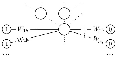
The synthetic nodes and edges need to be added to prevent the label propagation algorithm from con-verging to the trivial solution that assigns r = 1to all points in the graph. This choice is theoretically motivated—a similarity graph for regression should have not only “sources” (good nodes with high value ofr) but also “sinks” (counterparts for the sources). Figure 1 illustrates the connections of a test node.

Similarity Measure The similarity measure used for comparing source and target sides is of prime importance, as it determines the structure of the graph. This has consequences for both computa-tional efficiency (denser graphs require more com-putation and memory) and the accuracy of the out-come. A low similarity threshold results in a rich graph with a large number of edges but possibly in-troduces noise. A higher threshold leads to a small graph emphasizing highly similar samples but with too many disconnected components. The similarity measure is also the means by which domain knowl-edge can be incorporated into the graph construc-tion process. Similarity may be defined at the level of surface word strings, but may also include lin-guistic information such as morphological features, part-of-speech tags, or syntactic structures. Here, we compare two similarity measures: the famil-iar BLEU score (Papineni et al., 2002) and a score based on string kernels. In using BLEU we treat each sentence as a complete document. BLEU is not symmetric—when comparing two sentences, differ-ent results are obtained depending on which one is considered the reference and which one is the hy-pothesis. For computing similarities between train and test translations, we use the train translation as

the reference. For computing similarity between two test hypotheses, we compute BLEU in both direc-tions and take the average. We note that more ap-propriate distance measures are certainly possible. Many previous studies, such as (Callison-Burch et al., 2006), have pointed out drawbacks of BLEU, and any other similarity measure could be utilized instead. In particular, similarity measures that model aspects of sentences that are ill handled by standard phrase-based decoders (such as syntactic structure or semantic information) could be useful here.

A more general way of computing similarity be-tween strings is provided by string kernels (Lodhi et al., 2002; Rousu and Shawe-Taylor, 2005), which have been extensively used in bioinformatics and email spam detection. String kernels map strings into a feature space defined by all possible sub-strings of the string up a fixed lengthk, and com-puting the dot product between the resulting feature vectors. Several variants of basic string kernels ex-ist, notably those allowing gaps or mismatches, and efficient implementations have been devised even for large scale applications. Formally, we define a sentencesas a concatenation of symbols from a fi-nite alphabetΣ(the vocabulary of the language) and an embedding function from strings to feature vec-tors,φ : Σ∗ → H. A kernel function K(s, t) com-putes the distance between the resulting vectors for two sentencessand t. In our case, the embedding function is defined as

φk_u(s) := X

i:u=s(i)

λ|i| u_∈Σk (5)

wherekis the maximum length of substrings,_|i_|is the length ofi, andλis a penalty parameter for each gap encountered in the substring.Kis defined as

K(s, t) =X

u

hφu(s), φu(t)iwu (6)

For the combination of source-side and target-side similarity scores (the function we denoted asκ) we test two simple schemes, using either the ge-ometric or the arithmetic mean of the individual scores. In the first case, large edge weights only re-sult when both source and target are close to each other; the latter may produce high edge weights when only one of them (typically the source score) is high. More sophisticated combination schemes, using e.g. weighted combination, could be used but were not investigated in this study.

Scalability Poor scalability is often mentioned as a drawback of graph-based learning. Straightfor-ward implementations of GBL algorithms often rep-resent the joint training and test data in working memory and therefore do not scale well to large data sets. However, we have developed several tech-niques to improve scalability without impeding ac-curacy. First, we construct separate graphs for each test sentence without losing global connectivity in-formation. The graph for a test sentence is com-puted as the transitive closure of the edge setEover the nodes containing all hypotheses for that test sen-tence. This smaller graph does not affect the out-come of the learning process for the chosen sentence because in label propagation the learned valuer(xi) can be influenced by that of another nodexj if and only if xj is reachable from xi. In the worst the-oretical case, the transitive closure could compre-hend the entire graph, but in practice the edge set is never that dense and can be easily pruned based on the heuristic that faraway nodes connected through low-weight edges have less influence on the result. We use a simple embodiment of this heuristic in a work-list approach: starting from the nodes of inter-est (hypotheses for the focal sentence), we expand the closure starting with the direct neighbors, which have the largest influence; then add their neighbors, which have less influence, and so forth. A thresh-old on the number of added vertices limits undue expansion while capturing either the entire closure or a good approximation of it. Another practical computational advantage of portioning work is that graphs for different hypothesis sets can be trivially created and used in parallel, whereas distributing large matrix-vector multiplication is much more dif-ficult (Choi, 1998). The disadvantage is that overall

1 0

1 0

. . . .

W2h

W1h 1−W1h

1_−W

2h

Figure 1: Connections for hypothesis nodexh.

Similar-ity edges with weightsWthlink the node with train

sen-tencesxt, for whichr(xt) = 1. For each of these edges

we define a dissimilarity edge of weight1₋Wth, linking

the node with nodex′tfor whichr(x′t) = 0. The vertex is

also connected to other test vertices (the dotted edges).

redundant computations are being made: incomplete estimates ofrare computed for the ancillary nodes in the transitive closure and then discarded.

Second, we obtain a reduction in graph size of or-ders of magnitude by collapsing all training vertices of the same r that are connected to the same test vertex into one and sum the edge weights. This is equivalent to the full graph for learning purposes.

3.2 Propagation

Label propagation proceeds as follows:

1. Compute the transitive closure over the edges starting from all hypothesis nodes of a given sentence.

2. On the resulting graph, collapse all test-train similarities for each test node by summing edge weights. Obtain accumulated similarities in row and column 1 of the similarity matrixW. 3. Normalize test-to-train_P weights such that

jW1j = P

jWj1 = 1.

4. Initialize the matrixPasPij = _1−Wi1W₊ijP

jWij.

(The quantity1₋W1iin the denominator is the weight of the dissimilarity edge.)

5. Initialize a column vector f of height n with

f1 = 1(corresponding to nodex1) and 0 in the remaining positions.

6. f′ ←P×f

7. Clampf₁′:f₁′ = 1

8. Iff′ _{∼=f, continue with step 11.}

9. f _←f′

10. Repeat from step 6.

Convergence Our algorithm’s convergence proof is similar to that for standard label propagation (Zhu, 2005, p. 6). We splitP as follows:

P =

0 PLU

PU L PU U

(7)

wherePU Lis a column vector holding global simi-larities of test hypotheses with train sentences,PLU is a horizontal vector holding the same similarities (though PLU 6= PU LT due to normalization), and

PU U holds the normalized similarities between pairs of test hypotheses. We also separatef:

f =

1

fU

(8)

where we distinguish the first entry because it repre-sents the training part of the data. With these nota-tions, the iteration formula becomes:

f_U′ =PU UfU +PU L (9)

Unrolling the iteration yields:

fU = lim n→∞

"

(PU U)nfU0 + n X

i=1

(PU U)i−1 !

PU L #

It can be easily shown that the first term converges to zero because of normalization in step 4 (Zhu, 2005). The sum in the second term converges to (I₋PU U)−1, so the unique fixed point is:

fU = (I−PU U)−1PU L (10)

Our system uses the iterative form. On the data sets used, convergence took 61.07 steps on average.

At the end of the label propagation algorithm, nor-malized scores are obtained for each N-best list (sen-tences without any connections whatsoever are as-signed zero scores). These are then used together with the other component models in log-linear com-bination. Combination weights are optimized on a held-out data set.

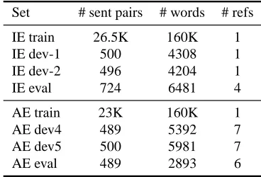
4 Data and System

We evaluate our approach on the IWSLT 2007 Italian-to-English (IE) and Arabic-to-English (AE) travel tasks. The first is a challenge task, where the

training set consists of read sentences but the de-velopment and test data consist of spontaneous di-alogues. The second is a standard travel expres-sion translation task consisting entirely of read in-put. For our experiments we chose the text input (correct transcription) condition only. The data set sizes are shown in Table 1. We split the IE develop-ment set into two subsets of 500 and 496 sentences each. The first set (dev-1) is used to train the system parameters of the baseline system and as a training set for GBL. The second is used to tune the GBL pa-rameters. For each language pair, the baseline sys-tem was trained with additional out-of-domain text data: the Italian-English Europarl corpus (Koehn, 2005) in the case of the IE system, and 5.5M words of newswire data (LDC Arabic Newswire, Multiple-Translation Corpus and ISI automatically extracted parallel data) in the case of the AE system.

Set # sent pairs # words # refs IE train 26.5K 160K 1 IE dev-1 500 4308 1 IE dev-2 496 4204 1

IE eval 724 6481 4

AE train 23K 160K 1

AE dev4 489 5392 7

AE dev5 500 5981 7

AE eval 489 2893 6

Table 1: Data set sizes and reference translations count.

Weighting dev-2 eval

none (baseline) 22.3/53.3 29.6/45.5 (a) 23.4/51.5 30.7/44.1 (b) 23.5/51.6 30.6/44.3 (c) 23.2/51.8 30.0/44.6

Table 2: GBL results (%BLEU/PER) on IE task for different weightings of labeled vs. labeled-unlabeled graph edges (BLEU-based similarity measure).

5 Experiments and Results

We started with the IE system and initially inves-tigated the effect of only including edges between labeled and unlabeled samples in the graph. This is equivalent to using a weightedk-nearest neighbor reranker that, for each hypothesis, computes average similarity with its neighborhood of labeled points, and uses the resulting score for reranking.

Starting with the IE task and the BLEU-based similarity metric, we ran optimization experiments that varied the similarity threshold and compared sum vs. product combination of source and target similarity scores, settling for θ = 0.7 and prod-uct combination. We experimented with three dif-ferent ways of weighting the contributions from labeled-unlabeled vs. unlabeled-unlabeled edges: (a) no weighting, (b) labeled-to-unlabeled edges were weighted 4 times stronger than unlabeled-unlabeled ones; and (c) labeled-to-unlabeled-unlabeled edges were weighted 2 times stronger. The weighting schemes do not lead to significantly different results. The best result obtained shows a gain of 1.2 BLEU points on the dev set and 1 point on the eval set, re-flecting PER gains of 2% and 1.2%, respectively.

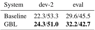
We next tested the string kernel based similarity measure. The parameter values were 0.5 for the gap penalty, a maximum substring length ofk= 4, and weights of 0, 0.1, 0.2, 0.7. These values were chosen heuristically and were not tuned extensively due to time constraints. Results (Table 3) show significant improvements in PER and BLEU.

In the context of the BTEC challenge task it is interesting to compare this approach to adding the development set directly to the training set. Part of the improvements may be due to utilizingkNN in-formation from a data set that is matched to the test

System dev-2 eval

Baseline 22.3/53.3 29.6/45.5 GBL 24.3/51.0 32.2/42.7

Table 3: GBL results (%BLEU/PER) on IE tasks with string-kernel based similarity measure.

set in terms of style. If this data were also used for training the initial phrase table, the improvements might disappear. We first optimized the log-linear model combination weights on the entire dev07 set (dev-1 and dev-2 in Table 1) before retraining the phrase table using the combined train and dev07 data. The new baseline performance (shown in Ta-ble 4) is much better than before, due to the im-proved training data. We then added GBL to this system by keeping the model combination weights trained for the previous system, using the N-best lists generated by the new system, and using the combined train+dev07 set as a train set for select-ing similar sentences. We used the GBL parameters that yielded the best performance in the experiments described above. As can be seen from Table 4, GBL again yields an improvement of up to 1.2% absolute in both BLEU and PER.

System BLEU (%) PER

Baseline 37.9 38.4

GBL 39.2 37.2

Table 4: Effect of GBL on IE system trained with matched data (eval set).

For the AE task we usedθ = 0.5; however, this threshold was not tuned extensively. Results using BLEU similarity are shown in Table 5. The best result on the eval set yields an improvement of 1.2 BLEU points though only 0.2% reduction in PER. Overall, results seem to vary with parameter settings and nature of the test set (e.g. on dev5, used as a test set, not for optimization, a surprisingly larger im-provement in BLEU of 2.7 points is obtained!).

con-Method dev4 dev5 eval

Baseline 30.2/43.5 21.9/48.4 37.8/41.8 GBL 30.3/42.5 24.6/48.1 39.0/41.6

Table 5: AE results (%BLEU/PER,θ= 0.5)

text. Since our similarity measure is word-based, this may cause similar sentences to fall below the threshold. The string kernel does not yield any im-provement over the BLEU-based similarity measure on this task. One possible improvement would be to use an extended string kernel that can take morpho-logical similarity into account.

Example Below we give an actual example of a translation improvement, showing the source sen-tence, the 1-best hypotheses of the baseline system and GBL system, respectively, the references, and the translations of similar sentences in the graph neighborhood of the current sentence.

Source: Al+ mE*rp Aymknk_{ltqAT Swrp lnA Baseline: i’m sorry could picture for us

GBL: excuse me could you take a picture of the us Refs:

excuse me can you take a picture of us excuse me could you take a photo of us pardon would you mind taking a photo of us pardon me could you take our picture pardon me would you take a picture of us excuse me could you take a picture of u Similar sentences:

could you get two tickets for us please take a picture for me

could you please take a picture of us 6 Related Work

GBL is an instance of semi-supervised learning, specifically transductive learning. A different form of semi-supervised learning (self-training) has been applied to MT by (Ueffing et al., 2007). Ours is the first study to explore a graph-based learning ap-proach. In the machine learning community, work on applying GBL to structured outputs is beginning to emerge. Transductive graph-based regularization has been applied to large-margin learning on struc-tured data (Altun et al., 2005). However, scalability quickly becomes a problem with these approaches; we solve that issue by working on transitive closures

as opposed to entire graphs. String kernel represen-tations have been used in MT (Szedmak, 2007) in a kernel regression based framework, which, how-ever, was an entirely supervised framework. Finally, our approach can be likened to a probabilistic imple-mentation of translation memories (Maruyana and Watanabe, 1992; Veale and Way, 1997). Translation memories are (usually commercial) databases of segment translations extracted from a large database of translation examples. They are typically used by human translators to retrieve translation candidates for subsequences of a new input text. Matches can be exact or fuzzy; the latter is similar to the iden-tification of graph neighborhoods in our approach. However, our GBL scheme propagates similarity scores not just from known to unknown sentences but also indirectly, via connections through other un-known sentences. The combination of a translation memory and statistical translation was reported in (Marcu, 2001); however, this is a combination of word-based and phrase-based translation predating the current phrase-based approach to SMT.

7 Conclusion

We have presented a graph-based learning scheme to implement a consistency model for SMT that encourages similar inputs to receive similar out-puts. Evaluation on two small-scale translation tasks showed significant improvements of up to 2.6 points in BLEU and 2.8% PER. Future work will include testing different graph construction schemes, in par-ticular better parameter optimization approaches and better string similarity measures. More gains can be expected when using better domain knowledge in constructing the string kernels. This may include e.g. similarity measures that accommodate POS tags or morphological features, or comparisons of the syntax trees of parsed sentence. The latter could be quite easily incorporated into a string kernel or the related tree kernel similarity measure. Additionally, we will investigate the effectiveness of this approach on larger translation tasks.

References

A. Alexandrescu and K. Kirchhoff. 2007. Data-Driven Graph Construction for Semi-Supervised Graph-Based Learning in NLP. In HLT.

Y. Altun, D. McAllester, and M. Belkin. 2005. Max-imum margin semi-supervised learning for structured variables. In Proceedings of NIPS 18.

A. Blum and S. Chawla. 2001. Learning from labeled and unlabeled data using graph mincuts. Proc. 18th International Conf. on Machine Learning, pages 19– 26.

C. Callison-Burch, M. Osborne, and P. Koehn. 2006. Re-evaluating the role of BLEU in machine translation re-search. In Proceedings of EACL.

Jaeyoung Choi. 1998. A new parallel matrix multi-plication algorithm on distributed-memory concurrent computers. Concurrency: Practice and Experience, 10(8):655–670.

A. Goldberg and J. Zhu. 2006. Seeing stars when there aren’t many stars: Graph-based semi-supervised learning for sentiment categorization. In HLT-NAACL Workshop on Graph-based Algorithms for Natural Language Processing.

T. Joachims. 2003. Transductive learning via spectral graph partitioning. In Proceedings of ICML.

Philipp Koehn, Hieu Hoang, Alexandra Birch, Chris Callison-Burch, Marcello Federico, Nicola Bertoldi, Brooke Cowan, Wade Shen, Christine Moran, Richard Zens, Chris Dyer, Ondrej Bojar, Alexandra Con-stantin, and Evan Herbst. 2007. Moses: Open source toolkit for statistical machine translation. In ACL. P. Koehn. 2005. Europarl: A parallel corpus for

sta-tistical machine translation. In Machine Translation Summit X, pages 79–86, Phuket, Thailand.

H. Lodhi, J. Shawe-taylor, and N. Cristianini. 2002. Text classification using string kernels. In Proceedings of NIPS.

D. Marcu. 2001. Towards a unified approach to memory-and statistical-based machine translation. In Proceed-ings of ACL.

H. Maruyana and H. Watanabe. 1992. Tree cover search algorithm for example-based translation. In Proceed-ings of TMI, pages 173–184.

Zheng-Yu Niu, Dong-Hong Ji, and Chew Lim Tan. 2005. Word sense disambiguation using label propagation based semi-supervised learning method. In Proceed-ings of ACL, pages 395–402.

K. Papineni, S. Roukos, T. Ward, and W. Zhu. 2002. Bleu: a method for automatic evaluation of machine translation. In Proceedings of ACL.

A. Ratnaparkhi. 1996. A maximum entropy part-of-speech tagger. In Proc.of (EMNLP).

J. Rousu and J. Shawe-Taylor. 2005. Efficient computa-tion of gap-weighted string kernels on large alphabets. Journal of Machine Learning Research, 6:1323–1344. A. Stolcke. 2002. SRILM—an extensible language

mod-eling toolkit. In ICSLP, pages 901–904.

Zhuoran Wang;John Shawe-Taylor;Sandor Szedmak. 2007. Kernel regression based machine translation. In Proceedings of NAACL/HLT, pages 185–188. Associ-ation for ComputAssoci-ational Linguistics.

Martin Szummer and Tommi Jaakkola. 2001. Partially labeled classification with markov random walks. In Advances in Neural Information Processing Systems, volume 14. http://ai.mit.edu/people/ szummer/.

N. Ueffing, G. Haffari, and A. Sarkar. 2007. Trans-ductive learning for statistical machine translation. In Proceedings of the ACL Workshop on Statistical Ma-chine Translation.

T. Veale and A. Way. 1997. Gaijin: a template-based bootstrapping approach to example-template-based ma-chine translation. In Proceedings of News Methods in Natural Language Processing.

X. Zhu and Z. Ghahramani. 2002. Learning from labeled and unlabeled data with label propagation. Technical report, CMU-CALD-02.