Abstract—In this study, we introduce a rapid iterative
algorithm to find a common element of the solution set of split variational inclusion problems and the set of fixed points of a nonexpansive mapping by using the hybrid steepest descent method. The strong convergence results of presented algorithms have been obtained under some mild conditions. The proposed results are the supplement, extension and generalization of the previously known results in this area. Finally, preliminary numerical results indicate the feasibility and efficiency of the proposed methods.
Index Terms—Split variational inclusion problem, Fixed
point problem, Nonexpansive mappings
I. INTRODUCTION
N 2011, A. Moudafi [1] first introduced the split monotone variational inclusion problem(SMVIP) as follow: Find a point x∗∈ H
1 such that
0 ∈ f1 x∗ + B1 x∗ (1) and
y∗= Ax∗∈ H
2 solves 0 ∈ f2 y∗ + B2 y∗ (2) whereH1 andH2 are two real Hilbert spaces with inner product ∙,∙ and induced norm ∙ , respectively. The mappings B1: H1→ 2H1and B
2: H2→ 2H2 are multi-valued maximal mappings.
A. Moudafi [1] revealed that SMVIP (1)-(2) included the split common fixed point problem, the split zero problem, the split variational inequality problem and split feasibility problem [1-8] as special cases, which have wide applications to intensity modulated radiation therapy treatment planning, see [6,7, 9,10].
If f1≡ 0 and f2≡ 0, then SMVIP (1)-(2) degenerate exactly into the split variational inclusion problem (SVIP): Look for x∗∈ H
1 such that
0 ∈ B1 x∗ (3)
Manuscript received June 06, 2015; revised July 28, 2015. This work was supported in part by the Natural Science Foundation of China (Grant No. 11401438, 11171180, 11171193, 11126233), the Natural Science Foundation of Shandong Province (Grant No. ZR2013FL032), and Project of Shandong Province Higher Educational Science and Technology Program (Grant No. J14LI52).
Haitao Che is with the School of Mathematics and Information Science, Weifang University, Weifang 261061, China. He is the corresponding author. (E-mail: [email protected])
Shoujin Li is with Weifang University of Science and Technology, Weifang 262700, China.
and
y∗= Ax∗∈ H
2 solves 0 ∈ B2 y∗ (4) We denote the solution set Γ of SVIP (3)-(4) by Γ = {x∗∈ H1: x∗∈ SOLVIP B
1 and Ax∗∈ SOLVIP B2 . }
Many works were devoted to SVIP (3)-(4) [4, 12, 14, 24, 25, 26, 27, 28]. In 2012, C. Byrne et al. [4] revealed the weak and strong convergence of the iterative method
xn+1= JλB1 x
n+ γA∗ Jλ
B2− I Ax
n (5) where A∗is the adjoint of A, and γ ∈ (0,2
L),λ > 0.
In 2014, Kazmi and Rizvi [12] proposed the following iterative procedure
un = JλB1 x
n+ γA∗ Jλ
B2− I Ax n
xn+1= anf(xn) + (1 − an)Sun) (6)
Then, the sequence xn converges strongly to the solution set Γ andthe fixed point of nonexpansive mapping S.
In 2015, using the hybrid steepest descent method, K. Sitthithakerngkietnet al. [14] considered theconvergence of the following iterative procedure
un= JλB1 x
n+ γA∗ Jλ
B2− I Ax n
xn+1= anf(xn) + (I − anD)Snun) (7)
where Sn is a sequence of nonexpansive mappings and D is a strongly positive bounded linear operator.
Following the work of Moudafi [1], Kazmi and Rizvi [12], Sitthithakerngkiet et al. [14], we introduce a rapid iterative algorithm for finding a common element of the solution set of split variational inclusion problems and the set of fixed points of a nonexpansive mapping. Under suitable conditions, the strong convergence for the sequences generated by the algorithm to a solution of the problems is proved. As applications, we apply our iterative algorithms to split feasibility problem. Preliminary numerical results indicate that our algorithm is more effective for SVIP (3)-(4) than the proposed algorithms in [4], [12] and [14].
II. PRELIMINARIES
Before proceeding further, we give a few concepts. A mappingT: H1→ H1 is called contraction, if there exists a constantα ∈ 0,1 such that
Tx − Ty ≤ α x − y , ∀ x, y ∈ H (8)
A Rapid Iterative Algorithm for Solving Split
Variational Inclusion Problems and Fixed Point
Problems
Haitao Che, Shoujin Li
I
IAENG International Journal of Applied Mathematics, 47:3, IJAM_47_3_01
holds.
If α = 1, then T is called nonexpansive.
A mapping T: H1→ H1 is said to be firmly nonexpansive, if
Tx − Ty, x − y ≥ Tx − Ty 2, ∀ x, y ∈ H
1 (9) A set-valued mappingQ: H1→ 2H1is called monotone if for all x, y ∈ H1,f ∈ Qx and g ∈ Qy imply x − y, f − g ≥ 0.
A monotone mapping Q: H1→ 2H1 is called maximal if the graph G(Q) of Q is not properly contained in the graph of any other monotone mapping. It is well known that a monotone mapping Q is maximal if and only if for the following relation x, f ∈ H × H, x − y, f − g ≥ 0, y, g ∈ G Q implies f ∈ Qx.
To obtain our results, we need the following technical lemmas.
Lemma 2.1 [18] If x, y, z ∈ H, then (a) x + y 2≤ x 2+ y, x + y .
(b) For any λ ∈ [0,1] λx + 1 + λ y 2= λ x 2+ 1 − λ y 2− λ 1 − λ x − y 2.
Lemma 2.2 [20] Assume that an is a sequence of nonnegative real numbers such thatan+1 ≤ 1 − γn an+ δn, n ≥ 0, where γn ∈ (0,1) and δn is a sequence inℝ, such that
(i) ∞ γn= ∞ n=0 (ii) limn→∞sup
δn
γn ≤ 0or δn< ∞ ∞
n=0
Then, limn→∞an= 0.
Lemma 2.3 [12] Assume A is a strongly positive linear bounded operator on a Hilbert space Hwith the coefficient
γ > 0and 0 < 𝜌 < A −1. Then I − ρA < 1 − 𝜌γ . III. MAINRESULTS
In this section, we first show some important lemmas and propose our algorithm. Then the convergence analysis of the algorithm is proved.
The following results are some important tools in this paper.
Lemma 3.1 [13] Let H be a real Hilbert space. LetM: H → 2H be a multi-valued maximal monotone mapping and let the resolving mappingJλM: H → H be defined byJλM x = I + λM −1(x) associated withM > 0, 𝜆 > 0. Then the following are satisfied:
(i) For eachλ > 0, JλMis a single-valued and firmly nonexpansive mapping.
(ii) Suppose that M−1(0) ≠ ∅ , then x − J λM(x)
2 + JλM(x) − x 2≤ x − x 2for eachx ∈ H, x ∈ M−1(0)andλ > 0.
(iii) Suppose thatM−1(0) ≠ ∅, then x − JλM x , J
λ
M x − w ≥ 0
foreachx ∈ H, w ∈ M−1(0)and 𝜆 > 0.
(iv) JλM(x) − JλM(y) 2≤ x − y, JλM x − JλM y for each x, y ∈ H and 𝜆 > 0.
Lemma 3.2 If the resolving mapping JλM: H → H is defined by Lemma 3.1, for each x, y ∈ H and 𝜆 > 0, then we have
(i) JλM x − JλM y 2≤ x − y 2− J λ
M x − x + y −
JλM y 2.
(ii) JλM x − x + y − J λ
M y ≤ x − y .
(iii) JλM x − x 2≤ JλM x − x, w − x ,for w ∈ M−1(0). Proof. For (i), from lemma 3.1 (iv), for x, y ∈ H, we have
JλM x − JλM y 2≤ x − y, J λ M x − J
λM y = x − y 2
+ x − y, JλM x − x + y − J λ M y
= x − y 2− J λ
M x − x + y − J λ M y 2
+ JλM x − JλM y , J
λM x − x + y − JλM y ≤ x − y 2− J
λ
M x − x + y − J λ M y 2.
(ii) is straightforward from (i), which means JλM x − x is 1-Lipschitz.
For (iii), from lemma 3.1 (iii), for x ∈ H one has
JλM x − x, w − x = J
λM x − x, w − JλM x + JλM x − x, J
λ
M x − x ≥ J λ
M x − x 2.
Lemma 3.3 [1]SVIP(3)-(4) is equivalent to the problem
x∗∈ H∗ such that y∗= Ax∗∈ H 2
x∗= J λ
B1x∗, y∗= J λ
B2y∗,for𝜆 > 0
Lemma 3.4 Let H1 and H2 be two real Hilbert spaces and
A: H1→ H1 be a bounded linear operator. Assume thatB1: H1→ 2H1and B2: H2→ 2H2 are maximal monotone mappings. Let S be a nonexpansive mappings on H1 such thatΓ ∩ F(S) ≠ ∅ . Supposef: H1→ H1 is a contraction mapping with constant β ∈ (0,1) and D is a strongly positive bounded linear operator with coefficient γ > 0and0 < 𝜉 <γ
β. For any t ∈ (0,1)andx ∈ H1 , let the mapping Wt on H1 be defined by Wtx = JλB1(I + τA∗(J
λ
B2− I)AJ λ
B1(tξf x + (I −
tD)Sx)where 𝜆 > 0, andτ ∈ (0, 1
L1), L1 is the spectral radius of the operator AA∗ and A∗ is the adjoint of A. Then the mapping Wt is contraction and has a unique fixed point.
Proof. Note that
JλB1(I + τA∗ J λ
B2− I A
is nonexpansive and I − tD ≤
1 − 𝑡γ . For any x, y ∈ H1 , we have
Wtx − Wty = Jλ B1(I
+ τA∗ J λ
B2− I A)J λ
B1 tξf x
+ I − tD Sx −JλB1(I + τA∗(J λ B2
− I)A)JλB1(tξf y + (I − tD)Sy)
≤ tξf x + I − tD Sx − (tξf y + (I − tD)Sy)
≤ tξβ x − y + (1 − 𝑡γ ) x − y = (1 − 𝑡(γ − ξβ)) x − y
Thus, Wt is a contraction whent ∈ (0, 1
γ −ξβ). Furthermore, it follows from the Banach contraction principle thatWt has a unique fixed point. This completes the proof.
IAENG International Journal of Applied Mathematics, 47:3, IJAM_47_3_01
Remark 3.1 Lemma 3.4 means that xt is the unique solution of the fixed point equationxt= JλB1(I + τA∗(J
λ B2−
I)AJλB1(tξf x
t + (I − tD)Sxt ).
Now, we are in a position to show the description of our algorithm.
Algorithm 3.1 For an arbitrary initial point x0∈ H1, we define {xn} by
yn = JλB1 a
nξf xn + (I − anD)Sxn xn+1= Jλ
B1 y
n+ τA∗(Jλ
B2− I)Ay n
(10)
where 𝜆 > 0,an ∈ (0,1), andτ ∈ (0,1
L1),L1 is the spectral radius of the operator AA∗ and A∗ is the adjoint of A.
Next, we will show the convergence analysis of the algorithm (10) for approximating a common solution of SVIP (3)-(4).
Theorem 3.1 Let H1 and H2 be two real Hilbert spaces and A: H1→ H1 be a bounded linear operator. Assume that
B1: H1→ 2H1 and B
2: H2→ 2H2 are maximal monotone mappings. Let S be a nonexpansive mappings onH1 . Let f: H1→ H2 be a contraction mapping with constant β ∈ (0,1)
and D be a strongly positive bounded linear operator with coefficient γ > 0 and 0 < 𝜉 <γ
β. Assume that Ω = Γ ∩ F(S) ≠ ∅. Let the sequences {xn} be generated by (10). Assume that the sequence {an} satisfies the following conditions:
(i) limn→∞an= 0. (ii) ∞n=0an= ∞.
(iii) ∞n=0 an+1− an < ∞.
Then {xn} converges strongly to a point z, where z = PΩ(I − D + ξf) is a unique solution of the variational inequalities
D − ξf z, z − x ≤ 0. (11) Proof. We divide the proof into five steps.
Step1.We prove that {xn} is bounded. Setp ∈ Ω. From p = JλB1p, Ap = J
λ
B2(Ap), Sp ∈ p, and Lemma 3.3, we have
xn+1− p 2= Jλ B1(y
n+ τA∗ Jλ
B2− I Ay n) − p
2 =
JλB1(y
n+ τA∗ Jλ
B2− I Ay n) − Jλ
B1p 2≤ y n+
τA∗ J λ
B2− I Ay n− p
2
= yn− p 2+ τ2 A∗ J λ B2−
I Ayn 2
+ 2τ yn− p, A∗ Jλ
B2− I Ay n (12) Since
2τ yn− p, A∗ Jλ
B2− I Ay
n = 2τ A yn− p , A∗ Jλ B2−
I Ayn = 2τ Ayn− Ap + JλB2− I Ay n − Jλ
B2−
I Ayn, JλB2− I Ay
n = 2τ Jλ B2Ay
n− p, Jλ
B2− I Ay n −
2τ JλB2− I Ay n
2
= τ JλB2Ay n− p
2
+ JλB2−
I Ayn 2− Ayn− Ap 2 − 2τ J λ
B2− I Ay n
2 ≤
τ JλB2− I Ay n
2
− 2τ JλB2− I Ay n
2
− 2τ JλB2−
I Ayn 2(13)
and
τ2 A∗ J λ
B2− I Ay n
2
= τ2 A∗ J λ
B2− I Ay n, A∗ Jλ
B2− I Ay n = τ2 J
λ
B2− I Ay
n, AA∗ Jλ
B2− I Ay
n ≤ L1τ2 Jλ B2−
I Ayn, JλB2− I Ay
n ≤ L1τ2 Jλ
B2− I Ay n
2
(14) From (13), (14) and (12), we deduce
xn+1− p 2≤ yn− p 2+ τ(L1τ − 1) Jλ
B2− I Ay n
2 ≤ yn− p 2 (15)
The definition of ynyields
yn− p = Jλ B1 a
nξf xn + I − anD Sxn − p ≤ anξf xn I − anD Sxn− p ≤ anξ f xn − f p + I − anD Sxn− p + an f p − Dp ≤ anξβ xn− p + (1 − anγ ) xn− p + an f p − Dp ≤ (1 − an(γ − ξβ) xn− p + an f p − Dp (16)
Thus, following from (15), (14) and Lemma 2.3, we have
xn+1− p ≤ yn− p ≤ (1 − an(γ − ξβ) xn− p + an f p − Dp ≤ max{ xn− p ,
f p −Dp
γ −ξβ (17) By induction, we have
xn+1− p ≤ max x0− p , f(p) − Dp γ − ξβ
which indicates that {xn} is bounded. It is easily to show that {f(xn)},{Sxn},{Dxn} and {yn} are all bounded.
Step 2. We reveal thatlimn→∞ xn+1− xn = 0. Since JλB1(I + λA∗(J
λ B2− I)A
is nonexpansive, one has
xn+1− xn = JλB1(I + τA∗ J λ
B2− I A) y n −Jλ
B1(I +
τA∗ J λ
B2− I A)y
n−1 ≤ yn− yn−1 (18)
In what follows, we will estimate yn− yn−1 . It follows from (10) that
yn− yn−1 = JλB1 a
nξf xn + I − anD Sxn −Jλ B1(a
n−1ξf xn−1 + (I − an−1D)Sxn−1) ≤ anξf xn + I − anD Sxn −
an−1ξf xn−1 + I − an−1D Sxn−1≤ anξβ xn− xn−1 + an− an−1 ξf xn−1 + 1 − anγ xn− xn−1 + an− an−1 DSxn−1 ≤ 1 − an γ − ξβ xn− xn−1 + an− an−1 ξf xn−1 + DSxn−1 (19)
Then, one has
xn+1− xn ≤ yn− yn−1
≤ 1 − an γ − ξβ xn− xn−1
+ an− an−1 ξf xn−1 + DSxn−1
Furthermore, by Lemma 2.2, we obtain
IAENG International Journal of Applied Mathematics, 47:3, IJAM_47_3_01
limn→∞ xn+1− xn = 0 (20) Step 3. We will obtainlimn→∞ Sxn− Sxn = 0.
Set zn= anξf xn + (I − anD)Sxn ). One has yn = JλB1z n. It follows from Lemma 2.1 that
yn− p 2= J λ B1 a
nξf xn + I − anD Sxn − p 2
≤ zn− p 2= anξf xn + I − anD Sxn− p 2= I − anD Sxn− I − anD p −anξf xn − anDp 2≤ I − anγ xn− p 2+ 2an ξf xn − Dp, zn− p ≤ xn− p 2+ 2an ξf xn − Dp zn− p (21)
(15) and (21) deduce
xn+1− p 2= yn− p 2+ τ(L1τ − 1) Jλ
B2− I Ay n
2
≤ I − anγ xn− p 2
+ 2an ξf xn − Dp zn− p + τ(L1τ − 1) JλB2− I Ay
n 2
≤ xn− p 2
+ 2an ξf xn − Dp zn− p + τ(L1τ − 1) JλB2− I Ay
n 2
Moreover,
τ(1 − L1τ) JλB2− I Ay n
2
≤ 2an ξf xn − Dp zn− p + ( xn− p 2 − xn+1− p 2)
≤ 2an ξf xn − Dp zn− p + xn− xn−1 xn− p + xn+1− p (22)
Sinceτ 1 − Lτ > 0,an → 0 and (22), we have limn→∞ (JλB2− I)Ay
n = 0 (23)
Furthermore, it follows from (10) that
xn+1− p 2= Jλ B1(y
n+ τA∗ Jλ
B2− I Ay n) − p
2
= JλB1(y
n+ τA∗ Jλ
B2− I Ay n) − Jλ
B1p 2
≤ xn+1− p, yn+ τA∗ Jλ
B2− I Ay n) − p
=1
2( xn+1− p 2
+ − xn+1− p − (yn+ τA∗ J λ
B2− I Ay n − p) 2=
1
2( xn+1− p 2+ y
n+ τA∗ Jλ
B2− I Ay n− p
2
− xn+1− yn− τA∗ Jλ
B2− I Ay n
2 )
≤1
2 xn+1− p 2 + y
n− p 2+ τ(Lτ
− 1) JλB2− I Ay n− p
2
− xn+1− yn− τA∗ J λ
B2− I Ay n
2 )
≤1
2( xn+1− p 2+ y
n− p 2
− ( xn+1− yn 2+ τ2 A∗ J λ
B2− I Ay n
2
− 2τ xn+1− yn, A∗ J λ
B2− I Ay n ))
≤1
2( xn+1− p 2+ y
n− p 2
− xn+1− yn 2
+ 2τ A xn+1− yn Jλ
B2− I Ay n )
which implies that
xn+1− p 2≤ yn− p 2− xn+1− yn 2+ 2τ A xn+1− yn JλB2− I Ay
n (24) Furthermore,
xn+1− yn 2≤ yn− p 2− xn+1− p 2+ 2τ A xn+1− yn JλB2− I Ay
n ≤ xn− p 2− xn+1− p 2+ 2an ξf xn − Dp yn− p + 2τ A xn+1− yn Jλ
B2−
I Ayn ≤ xn− xn−1 xn− p − xn+1− p + 2an ξf xn − Dp yn− p + 2τ A xn+1− yn Jλ
B2−
I Ayn (25) Following the fact an→ 0 and (20), (23), we have
limn→∞ xn+1− yn = 0 (26)
which means that
limn→∞ xn− yn = 0 (27)
Since I − JλB2 is a firmly nonexpansive mapping, we obtain
I − JλB2 Ax
n− I − Jλ B2 Ay
n
≤ Axn− Ayn, I − JλB2 Ax n − I − JλB2 Ay
n ≤ xn− yn, A∗ I − J
λ B2 Ax
n − A∗ I − J
λ B2 Ay
n ≤ xn− yn A∗ I − Jλ
B2 Ax n − A∗ I − J
λ B2 Ay
n
Thus,
lim n→∞ I − Jλ
B2 Ax
n− I − Jλ B2 Ay
n = 0
This together with (23) implies
IAENG International Journal of Applied Mathematics, 47:3, IJAM_47_3_01
limn→∞ I − Jλ B2 Ax
n = 0 (28)
On the other hand, we note that
xn+1− JλB1y
n ≤ Jλ B1 y
n+ τA∗ Jλ
B2− I Ay n − Jλ
B1y n ≤ (yn+ τA∗ Jλ
B2− I Ay n) − yn = τA∗ J
λ
B2− I Ay n ≤ τ A∗ J
λ
B2− I Ay n
And
xn− Jλ B1x
n ≤ xn− xn+1+ xn+1− Jλ B1y
n + JλB1y
n−Jλ B1x
n
≤ xn− xn+1 + xn+1− JλB1y n + JλB1y
n−Jλ B1x
n
From (20), (23) and (27), we have
limn→∞ xn− Jλ B1x
n = 0 (29) It follows from lemma 3.1 and (21) that
yn− p 2= Jλ B1 a
nξf xn + I − anD Sxn − p 2
=
JλB1z n− p
2
≤ zn− p 2− Jλ B1z
n− zn 2
=
zn− p 2− yn− zn 2≤ xn− p 2+ 2an ξf xn − Dp zn− p − yn− zn 2 (30)
Therefore,
xn+1− p 2≤ yn− p 2 ≤ xn− p 2
+ 2an ξf xn − Dp zn− p − yn− zn 2
Furthermore,
yn− zn 2≤ xn− p 2− xn+1− p 2 + 2an ξf xn − Dp zn− p
≤ xn− xn+1 xn− p + xn+1− p + 2an ξf xn − Dp zn− p
which means that
limn→∞ yn− zn = 0 (31) Consequently,
lim
n→∞ xn− zn
≤ limn→∞( xn− yn + yn− zn ) = 0 (32)
Since
zn− Sxn = anξf xn + I − anD Sxn− Sxn = an ξf xn − DSxn
Bya → 0, we have
limn→∞ zn− Sxn = 0 (33) By (32), one has
limn→∞ Sxn− xn = 0 (34)
Step 4. Next, we will prove that
limn→∞sup D − ξf z, z − yn ≤ 0 (35)
To obtain this inequality, we need to show the following inequality limn→∞sup D − ξf z, z − xn ≤ 0 holds, wherez = PΩ I − D + ξf (z) is a unique solution of the variational inequality (11).
We choose a subsequence {xnj} of {xn} such that
lim
n→∞sup D − ξf z, z − xn = limj→∞sup D − ξf z, z − xnj
Since {xnj} is bounded, then there exists a subsequence
{xnjk} of {xnj} which converges weakly to q. Without loss of generality, we assume thatxnj → q. Thus, from (28), (29) and (34), we obtainq ∈ Ω. Since z = PΩ I − D + ξf z, it follows that
limn→∞sup D − ξf z, z − xn = limj→∞sup D − ξf z, z − xnj = D − ξf z, z − q ≤ 0.
This together with (27) means that (35) holds. Step 5. Finally, we show that xn→ z.
Indeed, from (10), we have
yn− z 2= Jλ B1z
n− z 2
≤ zn− z, Jλ B1z
n− z = zn− z, yn− z
= anξf xn + I − anD Snxn− z, yn− z + an ξf z − Dz, yn− z
≤ (1 − an(γ − ξβ)) xn− z yn− z + an ξf z − Dz, yn− z
≤(1 − an(γ − ξβ))
2 xn− z
2+1
2 yn− z 2
+ an ξf z − Dz, yn− z
It follows that
yn− z 2≤ (1 − an(γ − ξβ)) xn− z 2+ 2an ξf z − Dz, yn− z (36)
From (36) and (10), we obtain
xn+1− z 2≤ yn− z 2
≤ (1 − an(γ − ξβ)) xn− z 2 + 2an ξf z − Dz, yn− z = (1 − an(γ − ξβ))
+2an(γ − ξβ)
(γ − ξβ) ξf z − Dz, yn− z
IAENG International Journal of Applied Mathematics, 47:3, IJAM_47_3_01
Hence, all conditions of Lemma 2.2 are satisfied, we immediately deduce thatxn → x. This completes the proof.
The following conclusions can be obtained from Algorithm 3.1 and Theorem 3.1 immediately.
Algorithm 3.2 For an arbitrary initial pointx0∈ H1, we define {xn} iteratively
yn= Jλ B1 a
nξf xn + (I − an)xn xn+1= JλB1 y
n+ τA∗(Jλ
B2− I)Ay n
(37)
Theorem 3.2 Let the sequences {xn} be generated by (37). Assume that the sequence {an} satisfies the control conditions:
(i) limn→∞an= 0. (ii) ∞n=0an= ∞.
(iii) ∞n=0 an+1− an < ∞.
Then, {xn} converges strongly to a pointz ∈ Γ, which solves the variational inequalities (11).
Algorithm 3.3 For an arbitrary initial pointx0∈ H1, we define {xn} iteratively by
yn = Jλ
B1 (I − a n)xn xn+1= JλB1 y
n+ τA∗(Jλ
B2− I)Ay n
(38) where 𝜆 > 0,an∈ [0,1], andτ ∈ (0,1
L1),L1is the spectral radius of the operator AA∗ and A∗ is the adjoint of A.
Theorem 3.3 Let the sequences {xn} be generated by (38). Assume that the sequence {an} satisfies the following conditions:
(i) limn→∞an= 0. (ii) ∞ an= ∞
n=0 .
(iii) ∞n=0 an+1− an < ∞.
Then, {xn} converges strongly to a point z ∈ Γ, which is the minimum norm element in Γ.
IV. APPLICATIONS
We now pay our attention to applying our iterative algorithms to split feasibility problem.
The split feasibility problem (SFP) was first introduced by Censor and Elfving [20] to look for
x ∈ C such that Ax ∈ Q (39) where A: H1→ H1 is a bounded linear operator, C and Q are nonempty closed convex subset of real Hilbert spaces H1 and
H2 , respectively. It is well known that SFP arise from phase retrievals and medical image reconstruction [21].
DefineB1= ∂δC: H1→ 2H1, where δC: H1→ [0, +∞]is the indicator function of C, i.e,
δC= 0, x ∈ C +∞, x ∉ C
andB2= ∂δQ: H2→ 2H2, where δQ: H2→ [0, +∞] is the indicator function of Q, i.e,
δQ =
0, x ∈ Q +∞, x ∉ Q
Thus, Algorithm 3.1 becomes to be the following algorithm.
Algorithm 4.1 For an arbitrary initial point x0∈ H1, we define {xn} iteratively by
yn = PC anξf xn + (I − anD)Sxn xn+1= PC yn+ τA∗(P
Q− I)Ayn
(40)
where 𝜆 > 0,an∈ [0,1], andτ ∈ (0,L1
1), L1 is the spectral radius of the operator AA∗ and A∗ is the adjoint of A.
Furthermore, if S = I, then Algorithm 4.1 can reduce to the following algorithm [22].
Algorithm 4.2 For an arbitrary initial pointx0∈ H1, we define {xn} iteratively by
yn = PC anξf xn + (I − anD)xn xn+1= PC yn+ τA∗(P
Q− I)Ayn
(41)
where 𝜆 > 0,an∈ [0,1], andτ ∈ (0,1
L1), L1 is the spectral radius of the operator AA∗ and A∗ is the adjoint of A.
V. NUMERICAL EXAMPLES
We now propose a numerical example to demonstrate the performance and the convergence of our result. In the experiment, the stopping criterion is xn− x∗ ≤ ε, IT denotes the iterative number, and SOL denotes a solution of the test problem. Setan=1
n,λ ∈ 0.5, ξ = 1,D = I, and the initial point(100,100)T.
Example 5.1 Let A and B1, B2: ℝ2→ ℝ2 be defined by A = 1 0
0 1 ,B1= 8 0
0 2 ,B2= 3 0 0 6
We take a mappingS: v = (v1, v2)T: → (sinv1, sinv2)T, and it is easily to see thatS is nonexpansive. Since1
L1= 1, so, we can take τ ∈ 0.8.
Example 5.2 Let A and B1, B2: ℝ2→ ℝ2 be defined by
A = 2 1
0 −1 ,B1= 8 0
0 2 ,B2= 3 0 0 6
Let S be the same as in Example 5.1. Since1
L1= 0.1910, so, we can takeτ ∈ 0.15.
Example 5.3 Let B1: ℝ2→ ℝ2 and B
2: ℝ3→ ℝ3 be defined by
A = 2 1 1 2 2 2
, B1= 8 00 2 ,B2=
3 0 0 0 6 0 0 0 9
We define a mapping S = 2 3
1 3 1 3
2 3
, and it is easy to observe that S is nonexpansive. Since1
L1= 0.0588, so, we can takeτ ∈ 0.05.
IAENG International Journal of Applied Mathematics, 47:3, IJAM_47_3_01
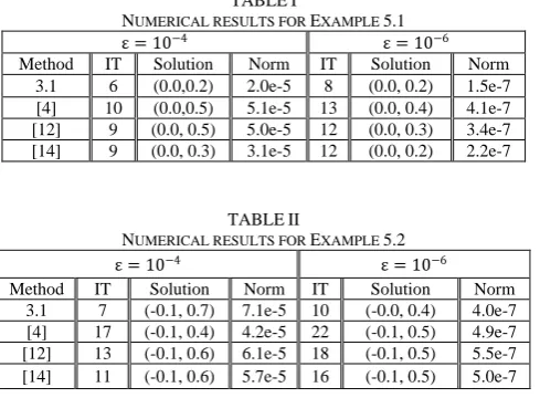
TABLEI
NUMERICAL RESULTS FOR EXAMPLE 5.1
ε = 10−4 ε = 10−6
Method IT Solution Norm IT Solution Norm 3.1 6 (0.0,0.2) 2.0e-5 8 (0.0, 0.2) 1.5e-7 [4] 10 (0.0,0.5) 5.1e-5 13 (0.0, 0.4) 4.1e-7 [12] 9 (0.0, 0.5) 5.0e-5 12 (0.0, 0.3) 3.4e-7 [14] 9 (0.0, 0.3) 3.1e-5 12 (0.0, 0.2) 2.2e-7
TABLEII
NUMERICAL RESULTS FOR EXAMPLE 5.2
ε = 10−4 ε = 10−6
Method IT Solution Norm IT Solution Norm 3.1 7 (-0.1, 0.7) 7.1e-5 10 (-0.0, 0.4) 4.0e-7 [4] 17 (-0.1, 0.4) 4.2e-5 22 (-0.1, 0.5) 4.9e-7 [12] 13 (-0.1, 0.6) 6.1e-5 18 (-0.1, 0.5) 5.5e-7 [14] 11 (-0.1, 0.6) 5.7e-5 16 (-0.1, 0.5) 5.0e-7
Table I, II and III at the initial point (10, 10) T with ε=1010 show that the iteration process of the sequence is a monotone decreasing sequence and the iteration sequence converges to (0, 0) T. Furthermore, it reveals that the more the iteration steps are, the more slowly the sequence converges to (0, 0) T. From Table I, II and III, we can observe that our algorithm is more effective for SVIP (3)-(4) than the proposed algorithms in [4], [12] and [14].
TABLEIII
NUMERICAL RESULTS FOR EXAMPLE 5.3
ε = 10−4 ε = 10−6
Method IT Solution Norm IT Solution Norm 3.1 6 (-0.0, 0.3) 3.2e-5 8 (-0.0, 0.2) 2.2e-7 [4] 14 (-0.2, 0.7) 6.8e-5 19 (-0.1, 0.4) 4.5e-7 [12] 11 (-0.2, 0.7) 7.7e-5 18 (-0.1, 0.4) 3.8e-7 [14] 9 (0.1, 0.1) 1.6e-5 11 (0.2, 0.4) 4.2e-7
REFERENCES
[1] A. Moudafi, “Split monotone variational inclusions,” Journal of Optimization Theory and Applications, Vol. 150, No.2, pp. 275–283, August 2011.
[2] Y. Censor, A. Gibali, and S. Reich, “Algorithms for the split variational inequality problem,” Numerical Algorithms, Vol.59, No.2, pp. 301-323, February 2012.
[3] A. Moudaf, “The split common fixed-point problem for demicontractive mapping,” Inverse Problems, vol.26, No.5, pp. 55007-55012, April 2010.
[4] C. Byrne, Y. Censor, A. Gibali, and S. Reich, “Weak and strong convergence of algorithms for the split common null point problem”,
Journal of Nonlinear and Convex Analysis, Vol. 13, No. 4, pp. 759-775, April 2012.
[5] X. Chi, Z. Wan, and Z. Hao, “The models of bilevel programming with lower level second-order cone programs,” Journal of Inequalities and Applications, Vol. 2014, No.1, pp.1-23, December 2014.
[6] Y. Censor, T. Bortfeld, B. Martin, and A. Trofimov, “A unified approach for inversion problems in intensity modulated radiation
therapy,” Physics in Medicine and Biology, Vol. 51, No. 10, pp. 2353-2365, April 2006.
[7] B. Qu, and N. Xiu, “A note on the CQ algorithm for the split feasibility problem,” Inverse Problems, Vol. 21, No, 5, pp. 1655-1665, September 2005.
[8] H. Che, and M. Li, “A simultaneous iterative method for split equality problems of two finite families of strictly pseudononspreading mappings without prior knowledge of operator norms,” Fixed Point Theory and Applications, Vol. 2015, No.1, pp. 1-14, December 2015. [9] C. Byrne, “Iterative oblique projection onto convex sets and the split
feasibility problem,” Inverse Problems, Vol. 18, No. 2, pp. 441-453, March2002.
[10] P. L. Combettes, “The convex feasibility problem in image recovery,”
Advances in Imaging and Electron Physics, Vol. 95, No. 8, pp. 155-270, 1996.
[11] P. Duan, and S. He, “Generalized viscosity approximation methods for nonexpansive mappings,” Fixed Point Theory and Applications, Vol. 2014, No. 1, pp. 1-11, December 2014.
[12] K. R. Kazmi, and S. H. Rizvi, “An iterative method for split variational inclusion problem and fixed point problem for a nonexpansive mapping,” Optimization Letters, Vol. 8, No. 3, pp. 1113-1124, March 2014.
[13] Z. He, and W. S. Du, “Nonlinear algorithms approach to split common solution problems,” Fixed Point Theory and Applications, Vol. 2012, No. 1, pp. 1-13, December 2012.
[14] K. Sitthithakerngkiet, J. Deepho, and P. Kumam, “A hybrid viscosity algorithm via modify the hybrid steepest descent method for solving the split variational inclusion in image reconstruction and fixed point problems,” Applied Mathematics and Computation, Vol. 250, pp. 986-1001, January 2015.
[15] H. K. Xu, “Averaged mappings and the gradient projection algorithm,”
Journal of Optimization Theory and Applications, Vol. 150, No. 2, pp. 360-378,August2011.
[16] K. Sakurai, and H. Iiduka, “Acceleration of the Halpern algorithm to search for a fixed point of a nonexpansive mapping,” Fixed Point Theory and Application, Vol. 2014, No. 1, pp. 1-11, Junuary 2014. [17] S. S. Chang, “Some problems and results in the study of nonlinear
analysis,” Nonlinear Analysis Theory Methods and Application, Vol. 30, No. 7, pp. 4197-4208, December. 1997.
[18] C. Byrne, “A unified treatment of some iterative algorithms in signal processing and image reconstruction,” Inverse Problems, Vol. 20, No. 1, pp. 103-120, February2004.
[19] H. K. Xu, “Viscosity approximation methods for nonexpansive mappings,” Journal of Mathematical Analysis and Applications, Vol. 298, No. 1, pp. 279-291, October 2004.
[20] Y. Yao, P. X. Yang, and S.M. Kang, “Composite projection algorithms for the split feasibility problem,” Mathematical and Computer Modelling, Vol. 57, No. 4, pp. 693-700, February 2013.
[21] M. M. Alves, and B. F. Svaiter, “A variant of the hybrid proximal extragradient method for solving strongly monotone inclusions and its complexity analysis,” Journal of Optimization Theory and Applications,Vol. 168, No. 1, pp. 198-215, January 2016.
[22] D. Li, and J. Zhao, “Monotone hybrid methods for a common solution problem in Hilbert spaces,” Journal of Nonlinear Science and Applications, Vol. 9, No. 3, pp. 757-765, September 2016.
[23] L. Rosasco, S. Villa, and B. C. Vũ, “Stochastic Forward–Backward Splitting for Monotone Inclusions,” Journal of Optimization Theory and Applications,Vol. 169, No. 2, pp. 388-406, May 2016.
[24] C. D. Enyi, and M. E. Soh, “Modified Gradient-Projection Algorithm for Solving Convex Minimization Problem in Hilbert Spaces,”
International Journal of Applied Mathematics, Vol. 44, No. 3, pp.144-150, July 2014.
[25] A. Cegielski, and F. Al-Musallam, “Strong convergence of a hybrid steepest descent method for the split common fixed point problem,”
Optimization, Vol. 65. No. 7, pp. 1463-1476, February 2016.