Performance Analysis of a Special GPIU Method for Singular Saddle Point Problems

(1)

Performance Analysis of a Special GPIU Method

for Singular Saddle Point Problems

Jae Heon Yun,

Member, IAENG

Abstract—In this paper, we first provide semi-convergence analysis for a special GPIU(Generalized Parameterized Inexact Uzawa) method with singular preconditioners for solving sin-gular saddle point problems. We next provide a methodology of how to choose nearly quasi-optimal parameters of the special GPIU method. Lastly, numerical experiments are carried out to examine the effectiveness of the special GPIU method with singular preconditioners by comparing its performance with that of other existing iterative methods for solving singular saddle point problems.

Index Terms—singular saddle point problem, GPIU method, semi-convergence, singular splitting, Moore-Penrose inverse.

I. INTRODUCTION

W

E consider the following large sparse augmented linear system

(

A B

−BT 0

) ( x y )

=

( f −g

)

, (1)

where A ∈Rm×m _{is a symmetric positive definite matrix,} and B ∈ Rm×n _{is a rank-deficient matrix with} _m _≥ _n_. In this case, the coefficient matrix of (1) is singular and so the problem (1) is called a singular saddle point problem. This type of problem appears in many different scientific applications, such as constrained optimization problems [13], [18], [30], the finite element approximation for solving the Navier-Stokes equation [10], the constrained least squares problems and generalized least squares problems [1], [24], and so on.

In case of B being of full rank, many relaxation it-erative methods have been proposed for solving the aug-mented linear system (1), e.g., SOR-like method [11], GSOR (Generalized SOR) method [2], PIU (Parameterized Inexact Uzawa) method [3], GPIU (Generalized Parame-terized Inexact Uzawa) method [7], the modified SOR-like method [16], SSOR-like method [8], the modified SSOR-like method [17], Uzawa-SAOR method [21], GSSOR (Gener-alized SSOR) method [25], and MIAOR (Modified inexact AOR) method [22].

Recently, several authors have presentedsemi-convergence analysis of relaxation iterative methods for solving the singular saddle point problem (1). Zheng et al [28] stud-ied semi-convergence of the PU (Parameterized Uzawa) method with nonsingular preconditioners, Li and Huang [14] examined semi-convergence of the GSSOR method with nonsingular preconditioners, Zhang et al. [26] provided semi-convergence analysis of the inexact Uzawa method with

Manuscript received April 7, 2017; revised June 15, 2017. This work was supported by Basic Science Research Program through the Na-tional Research Foundation of Korea(NRF) funded by the Ministry of Education(NRF-2016R1D1A1A09917364).

Jae Heon Yun (Corresponding author) is with the Department of Mathematics, College of Natural Sciences, Chungbuk National University, Cheongju 28644, Korea e-mail: [email protected].

nonsingular preconditioners, Zhang and Wang [27] stud-ied semi-convergence of the GPIU method with nonsin-gular preconditioners, Chao and Chen [6] provided semi-convergence analysis of the Uzawa-SOR method with non-singular preconditioners, Zhou and Zhang [29] studied semi-convergence of the GMSSOR (Generalized Modified SSOR) method with nonsingular preconditioners, Yun [23] studied acceleration of one-parameter relaxation methods with non-singular preconditioners, Liang and Zhang [15] presented semi-convergence analysis of the Uzawa-SAOR method with singular or nonsingular preconditioners, Yang et al. [20] pre-sented semi-convergence analysis of the Uzawa-HSS method with singular preconditioners, Yang et al. [19] presented semi-convergence analysis of the PIU method with singular preconditioners, and so on.

The purpose of this paper is to provide performance analysis of a special case of the GPIU method with singular preconditioners for solving the singular saddle point prob-lem (1). This paper is organized as follows. In Section 2, we provide preliminary results for semi-convergence analysis of the basic iterative methods. In Section 3, we provide semi-convergence results for a special case of the GPIU method with singular preconditioners. In Section 4, we first provide a methodology of how to choose nearly quasi-optimal pa-rameters of the special GPIU method, and then we provide numerical experiments in order to examine the effectiveness of the special GPIU method with singular preconditioners. Lastly, some conclusions are drawn.

II. PRELIMINARIES FORSEMI-CONVERGENCE ANALYSIS

For simplicity of exposition, some notation and definitions are presented. For a vector x, x∗ denotes the complex conjugate transpose of the vectorx.λmin(H)andλmax(H) denote the minimum and maximum eigenvalues of the Her-mitian matrixH, respectively. For a square matrixG,R(G) denotes the range space ofG,N(G)denotes the null space ofG,σ(G)denotes the set of all eigenvalues ofG, andρ(G) denotes the spectral radius ofG.

Let us recall some useful results on iterative methods for solving singular linear systems based on matrix splitting. For a matrixE∈Rn×n_{, the smallest nonnegative integer}_k_such thatrank(Ek)= rank(Ek+1)is called theindexofE, and denoted byk=index(E). In other words,index(E)is the size of the largest Jordan block corresponding to the zero eigenvalue ofE. For a square matrxT, thepseudo-spectral radiusν(T)is defined by

ν(T) = max{|λ| |λ∈σ(T)− {1}}

whereσ(T)is the set of eigenvalues of T.

The Moore-Penrose inverse [4] of a singular matrix E∈ Rn_×n _{is defined by the unique matrix}_E_†_{which satisfies the}

IAENG International Journal of Applied Mathematics, 47:3, IJAM_47_3_14

(2)

following equations

E=EE†E, E†=E†EE†, (EE†)T=EE†, (E†E)T =E†E.

LetA=M−Nbe a splitting of a singular matrixA, where

M is singular. Then an iterative method corresponding to this singular splitting for solving a singular linear systemAx=b

is given by

xi+1= (I−M†A)xi+M†b for i= 0,1, . . . . (2)

Definition 2.1: The iterative method (2) is semi-convergentif for any initial guessx0, the iteration sequence {xi} produced by (2) converges to a solution x_∗ of the singular linear system Ax=b.

Notice that a matrix T is called semi-convergent if lim

k→∞T

k _{exists, or equivalently} _index₍_I ₋_T_{) = 1} _and

ν(T)<1 [4].

Theorem 2.2 ([5]): The iterative method (2) is semi-convergent if and only ifindex(M†A) = 1,ν(I−M†A)<

1, andN(M†A) =N(A), i.e.,I−M†Ais semi-convergent andN(M†A) =N(A).

III. SEMI-CONVERGENCE ANALYSIS OF A SPECIALGPIU METHOD

In this section, we provide semi-convergence analysis for a special case of the GPIU method withsingular precondition-ers for solving the singular saddle point problem (1). Notice that Chen and Jiang [7] presented convergence analysis of the GPIU method for nonsingular saddle point problems, and Zhang and Wang [27] provided semi-convergence analysis of the GPIU method with nonsingular preconditioners for the singular saddle point problem (1).

Assume that the coefficient matrix Aof (1) is split as

A=

(

A B

−BT ₀ )

=D − L − U, (3)

where D= ( P 0 0 Q )

,L= (

0 0

BT 0 )

, U= (

P−A −B

0 Q

)

, (4)

where P ∈Rm×m _{is a symmetric positive definite (SPD)} matrix which approximates A, andQ∈Rn×n _{is a singular} symmetric positive semi-definite matrix which approximates the approximated Schur complement matrix BT_P−1_B_{. Let}

s be a real parameter andQ be chosen asQ=BTM−1B, where M is a SPD matrix which approximates P. Then a special case of the GPIU method with the singular precon-ditioning matrix Q, which is called the SGPIU method, is defined by

(

xk+1 yk+1

)

=H4(s) (

xk yk

) +M4(s)

(

f

−g

)

, k= 0,1,2, . . . , (5)

where

H4(s) =I−(D+ (s−1)L)†A

M4(s) = (D+ (s−1)L)†.

By some manipulation, one obtains

M4(s) = (

P−1 ₀

(1−s)Q†BTP−1 Q†

)

(6)

and

H4(s) = (

Im−P−1A −P−1B Q†BT(Im+ (s−1)P−1A) In+ (s−1)Q†BTP−1B

) .

(7)

From (5), (6) and (7), the SGPIU method with the singu-lar preconditioner Q for solving the singular saddle point problem (1) can be rewritten as

Algorithm 1: SGPIU method with singularQ Choosesand initial vectorsx0, y0

Fork= 0,1, . . . ,until convergence

xk+1=xk+P−1(f −Axk−Byk)

yk+1=yk+Q†(BTxk+1−g−sBT(xk+1−xk))

=yk+Q†(BT((1−s)xk+1+s xk)−g) End For

If s = 0, P is replaced by _ω1P with ω ∈ (0,2) and Q is replaced by_τ1Qwithτ >0, then the SGPIU method reduces to the PIU method. In particular, ifs= 0, P = _ω1Aand Q

is replaced by 1_τQ, then the SGPIU method reduces to the PU method.

Assume that the rank of B isr, i.e., r =rank(B)< n. Let

B=WΣV∗ and Σ =

(

Σr 0

0 0

)

∈Rm_×n ₍₈₎

be the singular value decomposition of B, where W and

V are unitary matrices, Σr = diag(σ1, σ2, . . . , σr) and σi’s are positive singular values of B. Let W and V be partitioned into W = (W1, W2) and V = (V1, V2) with

W1 ∈ Cm×r, W2 ∈ Cm×(m−r), V1 ∈ Cn×r, V2 ∈

Cn×(n−r)_{, respectively. Let us define an}₍_m₊_n₎_×₍_m₊_n₎

unitary matrixP as

P = ( W 0 0 V ) . (9)

Let Hˆ4(s) = P∗H4(s)P. If we define Pˆ =W∗P W,Aˆ =

W∗AW, andQˆ=V∗QV. Since Q=BT_M−1_B _and_B ₌

WΣV∗, one can obtain

ˆ

Q=V∗QV =

(_ˆ Q1 0

0 0

)

, (10)

whereQˆ1= ΣrW1∗M−1W1Σris anr×rSPD matrix. Thus

ˆ

Q†=V∗Q†V =

(_ˆ Q−₁1 0

0 0

)

(11)

and

ˆ

H4(s) = (

Im−Pˆ−1Aˆ −Pˆ−1Σ

ˆ

Q†ΣT₍_I

m+ (s−1) ˆP−1Aˆ In+ (s−1) ˆQ†ΣTPˆ−1Σ )

.

(12)

If we letB1=

(

Σr

0

)

∈Rm×r_{, then using (10) to (12)}

ˆ H4 (s) =

  

Im−P−1 ˆˆ A −P−ˆ 1_B

1 0

ˆ

Q−1₁ BT_{1 (}Im+ (s−1) ˆP−1 ˆA Ir+ (s−1) ˆQ−1₁ BT₁Pˆ−1B1 0

0 0 _In−r

  

(13)

andQˆ1=BT1(W∗M−1W)B1. If we let

¯

H(s) =

(

Im−Pˆ−1Aˆ −Pˆ−1B1

ˆ

Q−1₁ B₁T(Im+ (s−1) ˆP−1Aˆ Ir+ (s−1) ˆQ−11 B T 1Pˆ−1B1

) ,

(14)

then H¯(s) is the iteration matrix of the SGPIU method applied to the following nonsingular saddle point problem

( _ˆ

A B1

−BT

1 0 ) ( ˆ x ˆ z ) = ( _ˆ f −gˆ

)

(15)

with the preconditioning matrixQˆ1andPˆ as an

approxima-tion ofAˆ.

IAENG International Journal of Applied Mathematics, 47:3, IJAM_47_3_14

(3)

Before proceeding to semi-convergence analysis of the SGPIU method for solving the singular saddle point prob-lem (1), we first consider convergence of the SGPIU method for solving the nonsingular saddle point problem (15) whose iteration matrix isH¯(s). Note thatB1has full column rank

r. From the convergence analysis described in [7], [27], one can easily obtain the following three lemmas.

Lemma 3.1: Letλbe an eigenvalue ofH¯(s)and

( ˆ x ˆ z ) be

the corresponding eigenvector. Thenλ̸= 1 andˆx̸= 0.

( ˆ x ˆ z ) be

the corresponding eigenvector. Thenλsatisfies the following quadratic equation

λ2+ ˆ

β−2 ˆα+ (1−s)ˆγ

ˆ

α λ+

ˆ

α−βˆ+sγˆ ˆ

α = 0,

whereαˆ =xˆ_x_ˆ∗∗Pˆxˆxˆ,βˆ= ˆ

x∗Aˆxˆ ˆ

x∗ˆx andˆγ=

ˆ

x∗B1Qˆ−11 B1Txˆ

ˆ

x∗xˆ .

( ˆ x ˆ z ) be

the corresponding eigenvector. Then|λ|<1 if and only if

ˆ

γ−4 ˆα+ 2 ˆβ <2sˆγ <2 ˆβ and γ >ˆ 0,

whereαˆ =xˆ_x_ˆ∗∗Pˆxˆxˆ,βˆ= ˆ

x∗Aˆxˆ ˆ

x∗ˆx andˆγ=

ˆ

x∗B1Qˆ−11 B T 1xˆ

ˆ

x∗xˆ .

Theorem 3.4: Let λ̸= 1be an eigenvalue of H4(s)and

( x y )

be the corresponding eigenvector. Then|λ|<1 if and

only if

γ−4α+ 2β <2sγ <2β and γ >0,

whereα=x_x∗_∗P x_x ,β= x_x∗_∗Ax_x andγ= x∗BQ_x_∗†_xBTx.

Proof: Since H4(s) and Hˆ4(s) are similar, λ is an

eigenvalue of Hˆ4(s). Since λ̸= 1, from (13) and (14) λis

also an eigenvalue ofH¯(s). Let

( ˆ x ˆ y )

be an eigenvector of

ˆ

H4(s)corresponding to the λ. Then

( ˆ x ˆ z )

is an eigenvector

of H¯(s) corresponding to the λ, where zˆ is the subvector consisting of the first r components ofyˆ. From the relation

ˆ

H4(s) = P∗H4(s)P, it is easy to show that xˆ = W∗x

and yˆ = V∗y. From Lemma 3.3, |λ| < 1 if and only if ˆ

γ−4 ˆα+ 2 ˆβ < 2sˆγ < 2 ˆβ and ˆγ > 0. Since xˆ = W∗x, ˆ

α=α and βˆ=β are immediately obtained. On the other hand,

x∗BQ†BTx=x∗BV Qˆ†V∗B∗x=x∗WΣ ˆQ†ΣTW∗x

=x∗W B1Qˆ−11B T

1W∗x= ˆx∗B1Qˆ− 1 1 B

T 1x.ˆ

(16)

From (16),ˆγ=γ is also obtained. Therefore, the proof is complete.

Corollary 3.5: Letλbe an eigenvalue ofH¯(s)and

( x y )

be an eigenvector ofH4(s)corresponding to the eigenvalue

λ. Then|λ|<1if and only if

γ−4α+ 2β <2sγ <2β and γ >0, (17)

whereα=x_x∗∗P xx ,β= x∗Ax

x∗x andγ=

x∗BQ†BT_x x∗x .

Proof: Since λ ̸= 1 from Lemma 3.1, this corollary follows from Theorem 3.4.

The following theorem shows that the conditionγ >0in (17) can be omitted.

Theorem 3.6: Letλ be an eigenvalue ofH¯(s)and

( x y )

be an eigenvector ofH4(s)corresponding to the eigenvalue

λ. Then|λ|<1 if and only if

γ−4α+ 2β <2sγ <2β, (18)

whereα= x_x∗∗P xx ,β= x∗Ax

x∗x andγ=

x∗BQ†BT_x x∗x .

Proof:From Theorem 3.4, it was shown thatαˆ=α >0, ˆ

β=β >0andγˆ=γ≥0. Ifγ= 0(i.e.,x∈N(BT)), then Lemma 3.2 implies that λ satisfies the following quadratic equation

λ2−(2−β

α)λ+ 1− β α = 0.

Since λ ̸= 1 from Lemma 3.1, λ = 1− β_α is obtained.

|λ|=|1−_αβ|<1is equivalent to β <2α, which is exactly the same condition as the inequality (18) for γ= 0. Hence this theorem follows from Corollary 3.5.

Theorem 3.7: Assume that2P−Ais symmetric positive definite. Thenρ( ¯H(s))<1if the following inequality holds

1 2 −

λmin(2P−A) ρ(BQ†BT₎ < s <

λmin(A) ρ(BQ†BT₎.

Proof: Since 2P −A is symmetric positive definite, 2α > β and thus the inequality (18) is true for all s when

γ = 0. Suppose that γ > 0. Then the inequality (18) is equivalent to

1 2−

2α−β γ < s <

β

γ. (19)

Hence, this corollary follows from Theorem 3.6 and the inequality (19).

Now we provide semi-convergence result for the SGPIU method for solving the singular saddle point problem (1).

Theorem 3.8: Assume that2P−Ais symmetric positive definite. Let Q=BT_M−1_B _{be a singular preconditioning}

matrix, where M is a SPD matrix which approximates P. Then the SGPIU method with the singularQfor solving the singular saddle point problem (1) is semi-convergent if the following inequality holds

1 2 −

λmin(2P−A) ρ(BQ†BT₎ < s <

λmin(A) ρ(BQ†BT₎.

Proof: By Theorem 3.7,ρ( ¯H(s)) <1. From (13) and (14), it is clear that the matrix Hˆ4(s) is semi-convergent.

Since Hˆ4(s) =P∗H4(s)P, H4(s)is also semi-convergent.

Notice that H4(s) = I −(D+ (s−1)L)†A. From

The-orem 2.2, we need to show that N(A) = N((D+ (s−

1)L)†A). Hence, it is sufficient to show that N((D+ (s−

1)L)†A) ⊂ N(A). Suppose that

( x y )

∈ N((D+ (s−

1)L)†A). Then

P−1₍_Ax₊_By_{) = 0} _and ₋_Q†_BT_x₊₍₁₋_s₎_Q†_BT_P−1₍_Ax₊_By_{) = 0}_.

From these equations, Ax+By = 0 and −Q†BT_x _{= 0}_.

SinceQQ†BT ₌_BT_{, one obtains} (

x y )

∈N(A). Therefore, the proof is complete.

Corollary 3.9: Let Pˆ be a SPD matrix which approx-imates A, P = _ω1Pˆ, Qˆ = BTM−1B and Q = _τ1Qˆ, where 0 < ω < 2, τ > 0 and M is a SPD matrix which approximatesP. Assume that2P−A is symmetric positive definite. Then the SGPIU method with the singular

IAENG International Journal of Applied Mathematics, 47:3, IJAM_47_3_14

(4)

Qfor solving the singular saddle point problem (1) is semi-convergent if the following inequality holds

1 2 −

λmin(ω2Pˆ−A)

τ ρ(BQˆ†BT₎ < s <

λmin(A)

τ ρ(BQˆ†BT₎.

Corollary 3.10: Let P = _ω1A, Qˆ =BT_M−1_B _and _Q₌ 1

τQˆ, where 0 < ω < 2, τ > 0 and M is a SPD matrix which approximates P. Then the SGPIU method with the singularQfor solving the singular saddle point problem (1) is semi-convergent if the following inequality holds

1 2 −

(

2

ω −1 )

λmin(A)

τ ρ(BQˆ†BT₎ < s <

λmin(A)

τ ρ(BQˆ†BT₎.

Proof:Since0< ω <2,2P−Ais symmetric positive definite. Hence this corollary follows from Corollary 3.9.

IV. NUMERICAL RESULTS

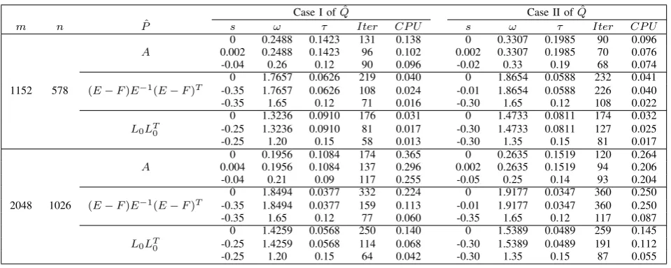
In this section, we first provide a methodology of how to choose nearly quasi-optimal parameters of the special GPIU method, and then we provide numerical experiments in order to examine the effectiveness of the SGPIU method with singular preconditioners for solving the singular saddle point problem (1). Performance of the SGPIU method with singular preconditioners is compared with that of the SGPIU method with nonsingular preconditioners and the PU or PIU methods with singular or nonsingular preconditioners.

In Tables II to V, Iter denotes the number of iteration steps, and CPU denotes the elapsed CPU time in seconds excluding the computational time of Q† for the singular case of Q or the Cholesky factorization time of Q for the nonsingular case of Q. In all experiments, the right hand side vector (fT_,₋_gT₎T _∈ _Rm+n _{was chosen such} that the exact solution of the saddle point problem (1) is (xT

∗, yT∗)T = (1,1, . . . ,1)T ∈ Rm+n, and the initial vector was set to the zero vector. All iterations for the singular saddle point problem are terminated if the current iteration satisfies RES<10−6_{, where} _RES_{is defined by}

RES=

√

∥f −Axk−Byk∥2+∥g−BTxk∥2 √

∥f∥2₊_∥_g_∥2 ,

where∥·∥denotes the L2-norm.

All numerical tests are carried out on a PC equipped with Intel Core i5-4570 3.2GHz CPU and 8GB RAM using MAT-LAB R2014b. For the elapsed CPU time, every experiment is repeated five times. The best and the worst ones out of 5 CPU times are discarded, and then the average of the remaining 3 CPU times is reported in Tables II to V.

Example 4.1 ([28]): We consider the saddle point prob-lem (1), in which

A=

(

I⊗T+T⊗I 0

0 I⊗T +T⊗I )

∈R2p2×2p2_,

B=(Bˆ B˜)=(Bˆ b1 b2

)

∈R2p2_×₍_p2₊₂₎

,

ˆ

B =

( I⊗F F⊗I

)

∈R2p2_×_p2

, b1= ˆB

( ep2_/₂

0

) ,

b2= ˆB

(

0

ep2_/₂

)

, ep2_/₂= (1,1, . . . ,1)T ∈Rp 2_/₂

,

T = 1

h2 ·tridiag(−1,2,−1)∈R

p_×p_,

F = 1

h·tridiag(−1,1,0)∈R p×p_,

with ⊗ denoting the Kronecker product and h = _p₊₁1 the discretization mesh size. For this example, m = 2p2 and

n=p2_{+ 2}_{. Thus the total number of variables is} ₃_p2_{+ 2}_.

Numerical results for this example are listed in Tables II and III.

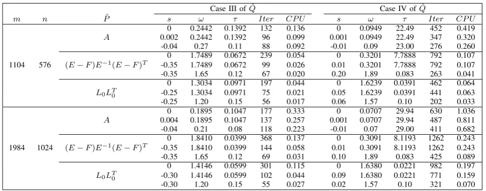
Example 4.2: Consider the Stokes equations of the fol-lowing form: finduandv such that

{

−△u+∇w=f inΩ

−∇ ·u= 0 inΩ, (20)

whereΩ = (0,1)×(0,1),uis a vector-valued function rep-resenting the velocity, andwis a scalar function representing the pressure. The boundary conditions areu= (0,0)T _{on the} three fixed walls (x= 0, y = 0, x= 1) and u= (1,0)T on the moving wall (y = 1). Dividing Ω into a uniform grid with mesh size h = 1_p and discretizing (20) by using MAC (marker and cell) finite difference scheme [9], [12], the singular saddle point problem (1) is obtained, where

A∈R2p(p−1)×2p(p−1)_{is a symmetric positive definite matrix}

andB=(Bˆ B˜)∈R2p(p−1)×p2 is a rank-deficient matrix of rank(B) = p2 −1 with Bˆ ∈ R2p(p−1)×(p2−1) and

˜

B∈R2p(p−1). For this example,m= 2p(p−1)andn=p2. Thus the total number of variables is3p2−2p. Numerical results for this example are listed in Tables IV and V.

For the SGPIU method, the symmetric positive definite matricesP are chosen asP =_ω1Pˆ with a positive parameter

ω ∈ (0,2) in three different ways. The first choice is ˆ

P =A, the second choice is Pˆ = (E−F)E−1(E−F)T, where A = E −F −FT is a splitting of the symmetric positive definite matrix A with E a diagonal matrix and

F a strictly lower triangular matrix, and the third choice is Pˆ = L0LT0, where A = L0LT0 −R0 is a splitting of

A obtained by an incomplete Cholesky factorization of A

with no fill-in. The singular or nonsingular preconditioning matricesQare chosen asQ= 1_τQˆ with a positive parameter

τ, where the matrices Qˆ are chosen as in Table I. In Table I, Diag( ˆBT_A_ˆ−1_B,_ˆ _B_˜T_B_˜₎ _{denotes a block diagonal matrix} consisting of two submatrices BˆT_A_ˆ−1_B_ˆ _and _B_˜T_B_˜_{. The} SGPIU algorithm for the nonsingular case ofQis the same as that for the singular case of Q except that Q−1 _{is used}

instead ofQ†.

For these choices ofPandQ, the SGPIU method withs= 0reduces to the PU method forP= _ω1Aor the PIU method for other two choices of P. For s = 0, the parameters ω

andτ are chosen as the optimal or quasi-optimal parameters which are computed using the formulas given in [28] or [19], respectively (see data reported in the first line of Tables II -V for each case ofPˆ). Fors̸= 0, the parameters are chosen in two different ways: One choice is thatωandτare chosen first as the optimal or quasi-optimal parameters and thens

is chosen as the best one by tries (see data reported in the second line of Tables II - V for each case ofPˆ), and the other choice is the experimentally chosen optimal parameterss,ω

andτ (see data reported in the third line of Tables II - V for each case ofPˆ). For singular matrixQ,Q† is computed only once using the Matlab function pinv with a drop tolerance 10−13, and then it is stored for later use. For nonsingular matrixQ, the Cholesky factorization of Qis computed only

IAENG International Journal of Applied Mathematics, 47:3, IJAM_47_3_14

(5)

[image:5.595.59.539.171.363.2]

TABLE I

CHOICES OFQˆFOR SINGULAR OR NONSINGULAR PRECONDITIONING MATRICESQ= 1_τQˆ

Case Number Qˆ Description Property ofQ

I BT_M−1_B _M₌_diag₍_A₎ _singular

II BT_M−1_B _M₌_tridiag₍_A₎ _singular

III Diag( ˆBT_Aˆ−1_B,ˆ _B˜T_B˜₎ _Aˆ₌_diag₍_A₎ _nonsingular

IV tridiag(Diag( ˆBT_Aˆ−1_B,ˆ _B˜T_B˜₎) _Aˆ₌_tridiag₍_A₎ _nonsingular

TABLE II

PERFORMANCE OFSGPIUMETHOD WITHP= _ω1PˆAND SINGULARQ=1_τQˆFOREXAMPLE4.1

Case I ofQˆ Case II ofQˆ

m n Pˆ s ω τ Iter CP U s ω τ Iter CP U

0 0.2488 0.1423 131 0.138 0 0.3307 0.1985 90 0.096

A 0.002 0.2488 0.1423 96 0.102 0.002 0.3307 0.1985 70 0.076

-0.04 0.26 0.12 90 0.096 -0.02 0.33 0.19 68 0.074

0 1.7657 0.0626 219 0.040 0 1.8654 0.0588 232 0.041

1152 578 (E−F)E−1₍_E₋_F₎T _-0.35 _1.7657 _0.0626 ₁₀₈ _0.024 _-0.01 _1.8654 _0.0588 ₂₂₆ _0.040

-0.35 1.65 0.12 71 0.016 -0.30 1.65 0.12 108 0.022

0 1.3236 0.0910 176 0.031 0 1.4733 0.0811 174 0.032

L0LT0 -0.25 1.3236 0.0910 81 0.017 -0.30 1.4733 0.0811 127 0.025

-0.25 1.20 0.15 58 0.013 -0.30 1.35 0.15 81 0.017

0 0.1956 0.1084 174 0.365 0 0.2635 0.1519 120 0.264

A 0.004 0.1956 0.1084 137 0.296 0.002 0.2635 0.1519 94 0.206

-0.04 0.21 0.09 117 0.255 -0.05 0.25 0.14 93 0.204

0 1.8494 0.0377 332 0.224 0 1.9177 0.0347 360 0.250

2048 1026 (E−F)E−1₍_E₋_F₎T _-0.35 _1.8494 _0.0377 ₁₅₉ _0.113 _-0.01 _1.9177 _0.0347 ₃₆₀ _0.250

-0.35 1.65 0.12 77 0.060 -0.35 1.65 0.12 117 0.087

0 1.4259 0.0568 250 0.140 0 1.5389 0.0489 259 0.145

L0LT0 -0.25 1.4259 0.0568 114 0.068 -0.30 1.5389 0.0489 191 0.112

-0.25 1.20 0.15 64 0.042 -0.30 1.35 0.15 87 0.055

TABLE III

PERFORMANCE OFSGPIUMETHOD WITHP= 1

ωPˆAND NONSINGULARQ=

1

τQˆFOREXAMPLE4.1

Case III ofQˆ Case IV ofQˆ

0 0.2489 0.1423 131 0.138 0 0.5622 2.9447 44 0.047

A 0.002 0.2489 0.1423 96 0.105 0.003 0.5622 2.9447 39 0.041

-0.04 0.25 0.13 91 0.096 -0.01 0.52 3.10 38 0.040

0 1.7657 0.0626 219 0.050 0 0.9617 1.8293 238 0.039

1152 578 (E−F)E−1₍_E₋_F₎T _-0.35 _1.7657 _0.0626 ₁₀₈ _0.028 _0.01 _0.9617 _1.8293 ₂₃₈ _0.039

-0.35 1.65 0.12 71 0.021 0.35 1.30 0.95 160 0.028

0 1.3236 0.0910 176 0.041 0 0.7849 1.8970 177 0.028

L0LT0 -0.25 1.3236 0.0910 81 0.022 0.01 0.7849 1.8970 177 0.028

-0.25 1.20 0.15 58 0.018 0.40 1.0 1.1 119 0.021

0 0.1956 0.1084 174 0.324 0 0.5115 3.3270 52 0.099

A 0.004 0.1956 0.1084 137 0.259 0.002 0.5115 3.3270 44 0.081

-0.04 0.21 0.09 117 0.221 -0.02 0.49 3.30 41 0.075

0 1.8494 0.0377 332 0.128 0 0.9580 1.8482 318 0.075

2048 1026 (E−F)E−1(E−F)T -0.35 1.8494 0.0377 159 0.065 0.01 0.9580 1.8482 318 0.075

-0.35 1.65 0.12 77 0.036 0.30 1.35 0.98 207 0.053

0 1.4259 0.0568 250 0.097 0 0.7844 1.9042 236 0.056

L0LT0 -0.25 1.4259 0.0568 114 0.048 0.01 0.7844 1.9042 236 0.056

-0.25 1.20 0.15 64 0.030 0.40 1.0 1.1 163 0.043

once using the Matlab functionchol, and then it is stored for later use.

For singular Q, Q†b is computed using matrix-times-vector operation after constructing Q† explicitly, which is very time-consuming. For nonsingular Q, Q−1_b _is

com-puted using the forward and backward substitutions after constructing the Cholesky factorization of Q explicitly. As can be seen in Tables II to V,P = _ω1L0LT0 provides better

performance and faster convergence rate than other two cases of P. From Tables II to V, it can be also seen that the SGPIU method with an appropriately chosen number sand optimal or quasi-optimal parametersωandτ performs better than the PU or PIU methods with optimal or quasi-optimal parameters ω andτ (i.e., the SGPIU methods with s= 0).

More specifically, when P = _ω1A, SGPIU method with an appropriately chosen numberscorresponding to optimal parametersωandτof the PU method performs significantly better than PU method with the optimal parametersω andτ

for all types of preconditionersQused in this paper. When

P = _ω1(E−F)E−1₍_E₋_F₎T _or 1

ωL0L T

0, SGPIU method

with an appropriately chosen number s corresponding to quasi-optimal parameters ω and τ of the PIU method per-forms much better than PIU method with the quasi-optimal parametersωandτ for the preconditionersQof types I and III. Clearly, the SGPIU method with experimentally chosen optimal parameterss,ω andτ performs best. However, we do not have a formula for finding optimal parameters of the SGPIU method, which should be done in the future work.

IAENG International Journal of Applied Mathematics, 47:3, IJAM_47_3_14

(6)

[image:6.595.57.539.73.266.2]

TABLE IV

PERFORMANCE OFSGPIUMETHOD WITHP= _ω1PˆAND SINGULARQ=1_τQˆFOREXAMPLE4.2

Case I ofQˆ Case II ofQˆ

0 0.2442 0.1392 132 0.136 0 0.3246 0.1939 89 0.096

A 0.002 0.2442 0.1392 96 0.099 0.002 0.3246 0.1939 73 0.082

-0.04 0.27 0.11 88 0.092 -0.04 0.32 0.18 69 0.075

0 1.7489 0.0672 239 0.042 0 1.8550 0.0634 255 0.044

1104 576 (E−F)E−1₍_E₋_F₎T _-0.35 _1.7489 _0.0672 ₉₉ _0.023 _-0.05 _1.8550 _0.0634 ₂₂₉ _0.041

-0.35 1.65 0.12 67 0.017 -0.35 1.65 0.12 110 0.024

0 1.3034 0.0971 197 0.034 0 1.4599 0.0871 196 0.037

L0LT₀ -0.25 1.3034 0.0971 75 0.018 -0.30 1.4599 0.0871 106 0.022

-0.25 1.20 0.15 56 0.014 -0.30 1.30 0.15 76 0.018

0 0.1895 0.1047 177 0.382 0 0.2555 0.1466 119 0.260

A 0.004 0.1895 0.1047 137 0.294 0.003 0.2555 0.1466 97 0.212

-0.04 0.21 0.08 118 0.259 -0.05 0.24 0.14 93 0.205

0 1.8410 0.0399 368 0.212 0 1.9127 0.0369 399 0.234

1984 1024 (E−F)E−1₍_E₋_F₎T _-0.40 _1.8410 _0.0399 ₁₃₇ _0.083 _-0.05 _1.9127 _0.0369 ₃₇₃ _0.217

-0.35 1.65 0.12 69 0.048 -0.35 1.65 0.12 116 0.072

0 1.4146 0.0599 301 0.180 0 1.5321 0.0517 293 0.172

L0LT0 -0.30 1.4146 0.0599 102 0.066 -0.35 1.5321 0.0517 150 0.093

-0.30 1.20 0.15 55 0.039 -0.30 1.35 0.15 78 0.052

TABLE V

PERFORMANCE OFSGPIUMETHOD WITHP=_ω1PˆAND NONSINGULARQ=1_τQˆFOREXAMPLE4.2

Case III ofQˆ Case IV ofQˆ

0 0.2442 0.1392 132 0.136 0 0.0949 22.49 452 0.419

A 0.002 0.2442 0.1392 96 0.099 0.001 0.0949 22.49 347 0.320

-0.04 0.27 0.11 88 0.092 -0.01 0.09 23.00 276 0.260

0 1.7489 0.0672 239 0.054 0 0.3201 7.7888 792 0.107

1104 576 (E−F)E−1₍_E₋_F₎T _-0.35 _1.7489 _0.0672 ₉₉ _0.026 _0.01 _0.3201 _7.7888 ₇₉₂ _0.107

-0.35 1.65 0.12 67 0.020 0.20 1.89 0.083 263 0.041

0 1.3034 0.0971 197 0.044 0 1.6239 0.0391 462 0.064

L0LT0 -0.25 1.3034 0.0971 75 0.021 0.05 1.6239 0.0391 441 0.063

-0.25 1.20 0.15 56 0.017 0.06 1.57 0.10 202 0.033

0 0.1895 0.1047 177 0.333 0 0.0707 29.94 630 1.036

A 0.004 0.1895 0.1047 137 0.257 0.001 0.0707 29.94 487 0.811

-0.04 0.21 0.08 118 0.223 -0.01 0.07 29.00 411 0.682

0 1.8410 0.0399 368 0.137 0 0.3091 8.1193 1262 0.243

1984 1024 (E−F)E−1₍_E₋_F₎T _-0.35 _1.8410 _0.0399 ₁₄₄ _0.058 _0.01 _0.3091 _8.1193 ₁₂₆₂ _0.243

-0.35 1.65 0.12 69 0.031 0.10 1.89 0.083 425 0.089

0 1.4146 0.0599 301 0.115 0 1.6380 0.0221 982 0.197

L0LT0 -0.30 1.4146 0.0599 102 0.044 0.09 1.6380 0.0221 771 0.159

-0.30 1.20 0.15 55 0.027 0.02 1.57 0.10 321 0.070

V. CONCLUSION

In this paper, we provided semi-convergence analysis of the SGPIU method with singular preconditioners for solv-ing ssolv-ingular saddle point problems. Numerical experiments show that the SGPIU method with an appropriately chosen numbers and optimal or quasi-optimal parametersω andτ

performs better than the PU or PIU methods with optimal or quasi-optimal parameters ω and τ. More specifically, when

P = 1

ωA, SGPIU method with an appropriately chosen number s corresponding to optimal parameters ω and τ

of the PU method performs significantly better than the PU method for all types of preconditioners Q used in this paper. When P = _ω1(E −F)E−1₍_E ₋_F₎T _or 1

ωL0L T

0,

SGPIU method with an appropriately chosen number s

corresponding to quasi-optimal parameters ω and τ of the PIU method performs about twice faster than the PIU method for the preconditionersQof types I and III. It means that the methodology of choosing an appropriate value of s

corresponding to the optimal or quasi-optimal parametersω

and τ of the PU or PIU methods works quite well for the SGPIU method.

It is clear that the SGPIU method with experimentally

cho-sen optimal parameterss,ω andτperforms best. So, further research for finding optimal parameters of the SGPIU method will be done in the future work. The SGPIU method with singular preconditioners performs rather well as compared with that with nonsingular preconditioners. However, the SGPIU method with singular preconditionersQrequires the computation ofQ†bfor a given vectorb, which is very time-consuming. Future work will also include how to compute

Q†befficiently for a given vector b.

ACKNOWLEDGMENT

The author is grateful to the anonymous reviewers for their valuable comments and suggestions which improved the quality and the clarity of the paper.

REFERENCES

[1] M. Arioli, I. S. Duff, P. P. M. de Rijk, ”On the augmented system approach to sparse least squares problems,”Numer. Math., vol. 55, pp. 667-684, 1989.

[2] Z.-Z. Bai, B. N. Parlett, Z.-Q. Wang, ”On generalized successive overrelaxation methods for augmented linear systems,”Numer. Math., vol. 102, pp. 1-38, 2005.

IAENG International Journal of Applied Mathematics, 47:3, IJAM_47_3_14

[image:6.595.57.540.302.492.2]

(7)

[3] Z.-Z. Bai, Z.-Q. Wang, ”On parameterized inexact Uzawa methods for generalized saddle point problems,”Linear Algebra Appl., vol. 428, pp. 2900-2932, 2008.

[4] A. Berman and R.J. Plemmons,Nonnegative matrices in the Mathemat-ical sciences, New York, Academic Press, 1979.

[5] Z.-H. Cao, ”On the convergence of general stationary linear iterative methods for singular linear systems,”SIAM J. Matyrix Anal. Appl., vol. 29, pp. 1382-1388, 2008.

[6] Z. Chao, G. Chen, ”Semi-convergence analysis of the Uzawa-SOR methods for singular saddle point problems,” Appled Mathematics Letters, vol. 35, pp. 52-57, 2014.

[7] F. Chen, Y.-L. Jiang, ”A generalization of the inexact parameterized Uzawa methods for saddle point problems,”Appl. Math. Comput., vol. 206, pp. 765-771, 2008.

[8] M. T. Darvishi, P. Hessari, ”Symmetric SOR method for augmented systems,”Appl. Math. Comput., vol. 183, pp. 409-415, 2006. [9] H. C. Elman, ”Preconditioning for the steady-state Navier-Stokes

equa-tions with low viscosity,”SIAM J. Sci. Comput., vol. 20, pp. 1299-1316, 1999.

[10] H. C. Elman, D. J. Silvester, ”Fast nonsymmetric iteration and pre-conditioning for Navier-Stokes equations,”SIAM J. Sci. Comput., vol. 17, pp. 33-46, 1996.

[11] G. H. Golub, X. Wu, J.-Y. Yuan, ”SOR-like methods for augmented systems,”BIT Numerical Mathematics, vol. 41, pp. 71-85, 2001. [12] F. H. Harlow and J. E. Welch, ”Numerical calculation of

time-dependent viscous incompressible flow of fluid with free surface,”Phys. Fluids, vol. 8, pp. 2182-2189. 1965.

[13] M. Keyanpour and A. Mahmoudi, ”A Hybrid Method for Solving Optimal Control Problems,” IAENG International Journal of Applied Mathematics, vol. 42, no. 2, pp80-86, 2012.

[14] J.-I. Li and T.-Z. Huang, ”The semi-convergence of generalized SSOR method for singular augmented systems,”Lecture Notes in Computer Science: High Performance Computing and Applications, vol. 5938, pp. 230–235, 2010.

[15] Z.-Z. Liang, G.-F. Zhang, ”On semi-convergence of a class of Uzawa methods for singular saddle point problems,”Appl. Math. Comput., vol. 247, pp. 397-409, 2014.

[16] X. Shao, Z. Li, C. Li, ”Modified SOR-like method for the augmented system,”Intern. J. Comput. Math., vol. 84, pp. 1653–1662, 2007. [17] S.-L. Wu, T.-Z. Huang, X.-L. Zhao, ”A modified SSOR iterative

method for augmented systems,”J. Comput. Appl. Math., vol 228, pp. 424-433, 2009.

[18] S. Wright, ”Stability of augmented system factorization in interior point methods,”SIAM J. Matrix Anal. Appl., vol. 18, pp. 191-222, 1997. [19] A.-L. Yang, Y. Dou, Y.-J. Wu, X. Li, ”On generalized parameterized inexact Uzawa methods for singular saddle point problems,” Numer. Algor., vol. 69, pp. 579-593, 2015.

[20] A.-L. Yang, X. Li, Y.-J. Wu, ”On semi-convergence of the Uzawa-HSS method for singular saddle point problems,”Appl. Math. Comput., vol. 252, pp. 88-98, 2015.

[21] J. H. Yun, ”Variants of the Uzawa method for saddle point problem,”

Comput. Math. Appl., vol. 65, pp. 1037-1046, 2013.

[22] J. H. Yun, ”Convergence of relaxation iterative methods for saddle point problem,”Appl. Math. Comput., vol. 251, pp. 65-80, 2015. [23] J. H. Yun, ”Acceleration of one-parameter relaxation methods for

singular saddle point problems,” J. Korean Math. Soc., vol. 53, pp. 691-707, 2016.

[24] J.-Y. Yuan, A. N. Iusem, ”Preconditioned conjugate gradient methods for generalized least squares problem,”J. Comput. Appl. Math., vol. 71, pp. 287-297, 1996.

[25] G.-F. Zhang, Q.-H. Lu, ”On generalized symmetric SOR method for augmented systems,”J. Comput. Appl. Math., vol. 219, pp. 51-58, 2008. [26] N.-M. Zhang, T.-T. Lu, Y. Wei, ”Semi-convergence analysis of Uzawa methods for singular saddle point problems,”J. Comput. Appl. Math., vol. 255, pp. 334-345, 2014.

[27] G.-F. Zhang, S.-S. Wang, ”A generalization of parameterized inexact Uzawa method for singular saddle point problems,”Appl. Math. Com-put., vol. 219, pp. 4225-4231, 2013.

[28] B. Zheng, Z.-Z. Bai, X. Yang, ”On semi-convergence of parameterized Uzawa methods for singular saddle point problems,”Linear Algebra Appl., vol. 431, pp. 808-817, 2009.

[29] L. Zhou, N.-M. Zhang, ”Semi-convergence analysis of GMSSOR methods for singular saddle point problems,”Comput. Math. Appl., vol. 68, pp. 596-605, 2014.

[30] M.-Z. Zhu, Y.-E. Qi, ”On the Eigenvalues Distribution of Precondi-tioned Block Two-by-two Matrix,” IAENG International Journal of Applied Mathematics, vol. 46, no. 4, pp500-504, 2016.