Boundedness Character of a Symmetric System
of Max-type Difference Equations
Chang-you Wang, Hao Liu,
Rui Li*
,Xiao-hong Hu
andYa-bin Shao
Abstract—This paper is concerned with the boundedness of the following symmetric system of max-type difference equations
1 1
1 1
max{ , }, max{ , }, ,
p p
n n
n q n q
n n
y x
0
x c y c n
x y
+ +
− −
= = ∈N
where , the parameters and the
initial conditions
{ }
0 0
N =N∪ c p q, , ∈(0, )∞
1, ,0 1, 0
x− x y− y are arbitrary positive real
numbers.
Index Terms—max-type system, difference equations, boundedness.
I. INTRODUCTION
iff an
erence equation appear naturally as discrete analogues d as numerical solutions of differential and delay differential equations, which have been applied in biology, ecology, physics, and so forth (see, [1-7]). Many researchers have studied the asymptotic behavior of the difference equation, for example, in [8, 9] and relevant references cited therein. Recently, the scholars have begun to pay more attention on the studying of so-called max-type difference equations. In the initial study, experts focused on studying the behavior of the following difference equation
(1) (2) ( )
0
1 2
max{ , , , },
k
n n n
n
n n n k
A A A
x n N
x− x− x−
= ∈ , (1)
wherek∈N, An( )i ,i=1, 2, ,k, are real sequences (mostly constant or periodic) and the initial values x−1,x−2, ,x−k are different from zero (see, [10, 11], as well as the references therein).
Elsayed et al. [12] have proved that every positive solution of the following third-order nonautonomous max-type difference equation
1 max{ n, } n
n
A x
x
+ = xn−2 (2) is periodic with period three whenAnis a three-periodic
Manuscript received March 13, 2016; revised May 25, 2016. This work is supported by Science Fund for Distinguished Young Scholars (cstc2014jc yjjq40004) of China, the National Nature Science Fund (Project nos.11372366 and 61503053) of China, the Science and Technology Project of Chongqing Municipal Education Committee (Grants no. kj1400423) of China, the Natural Science Foundation Project of CQ CSTC (CSTC, cstc2015jjA20016) of China, and the excellent talents project of colleges and universities in Chongqing of China.
Chang-you Wang, Hao Liu, and Rui Li are with Key Laboratory of Network control & Intelligent Instrument (Chongqing University of Posts and Telecommunications), Ministry of Education, Chongqing 400065, P.R.
China. (*Corresponding Author: E-mail Address: [email protected]).
Chang-you Wang, Xiao-hong Hu and Ya-bin Shao are with College of Science, Chongqing University of Posts and Telecommunications, Chongqing 400065 P. R. China.
sequence of positive numbers.
In [13], Xiao et al. have shown that every well-defined solution of the following difference equation
n 1 max{ , n1}, n
0
x x n N
x β
+ = − ∈ (3)
is eventually periodic with period two, where the initial conditions x−1,x0 are arbitrary non-zero real numbers andβ∈R.
In 2008, S. Stević [14] proposed some open problem and suggested investigation of positive solutions to the following difference equation
1 2
1 2
1 2
1 2
(0) (1) (2) ( )
0
max{ , , , , },
k k k
k
r
r r
n p
n p n p k
n n n s n s n s
n q n q n q
x
x x
x B B B B n N
x x x
−
− −
− − −
= ∈
(4) wherep qi, iare natural numbers such that p1< p2 < < pk,
1 2 k
q <q < <q , r si, i∈R+, is a sequence of positive numbers,
( )i n B 1, 2, ,
i= kandk∈N.
As a special case of Equation (4), S. Stević studied the boundedness character of positive solutions to the following max-type difference equation
1
0
max{ , },
p n
n r
n k x
x A n
x
− −
= ∈N , (5) where , the parameters and are positive and is a nonnegative real number (see, [15]).
\{1}
k∈N A r
p
In view of a natural extension of the model (5), S. Stević
continuously investigated the behavior of positive solutions to the following max-type system of differences
1 1
1 1
max{ , }, max{ , },
p p
n n
n p n p
n n
y x
0
x c y c n
x y
+ +
− −
= = ∈N
d
, (6) where the parameters c an pare positive real numbers. And who proved that all positive solutions of system (6) are bounded when and so forth (see [16]). In addition, related research can also be seen in papers [17-20] and the references therein.
(0, 4)
p∈
In this paper, based on the idea of works [14-16], we study the boundedness character of the following max-type difference equations
1 1
1 1
max{ , }, max{ , },
p p
n n
n q n q
n n
y x
0
x c y c n
x y
+ +
− −
= = ∈N (7)
where c p q, , ∈(0,+∞) and the initial conditions x−1, ,x y0 −1,
0
y are arbitrary positive real numbers.
II. BOUNDEDNESS CHARACTER OF SOLUTIONS
In this section, we will analyze the boundedness of the
D
IAENG International Journal of Applied Mathematics, 46:4, IJAM_46_4_14
positive solutions to system (7).
Theorem 1. Assume that f( )λ λ= 2−pλ+q and (a) there is λ1>1such that f( ) 0λ1 = , or (b) there is λ λ1= 2=1 such that f( )λ1 =f( ) 0λ2 = , then the system (7) has positive unbounded solutions with the positive initial conditions
1
,
1, ,
0 0x
−y
−x y
such thatx y
0 0>
x y
− −1 1>
0
.Proof. Obviously, from (7), we can easily see that
1 1
1 1
,
p p
n
n q n
n n y x x y x y + + − −
≥ ≥ n
q
1 n . (8) By taking logarithm in (8), for anyn∈N0, we obtain
1 1 1
lnxn+ ≥ plnyn−qlnxn−, lnyn+ ≥ plnxn−qlny−
−
n
y
0
. (9) Moreover, it follows that
lnxn+1yn+1≥ plnx yn n−qlnxn−1yn−1,n≥ 1. (10) Letzn =lnxn , then inequality (10) becomes
1 1,
n n n
z + ≥ pz −qz − n∈N . (11) By hypothesis (a), we have that f( ) 0λ1 = and λ1>1.
Let
1
1 ( ) ( ) f
f λ λ a
λ λ
= =
− λ+ , (12) then it follows that
1
( ) ( )( )
f λ = λ+a λ λ− . (13) Comparing Eq. (12) with Eq. (13), we can obtain a=λ1−p and q= −aλ1.
Set
-1, 0
n n n
u =z +az n∈N . (14) Then inequation (11) can be written in the following form
(15)
1 1 1 1
1 1
1 1
( )
( )
0.
n n n n n
n n n n
n n
z pz qz z a z a z
z az z az
u u λ λ λ λ + − + + + − + = − − + = + − + = − ≥ 2 1 1 n− − n u That is
un+1≥λ1 . (16) Let z−1,z0 be chosen such that
0 | || |
z ≥ a z−1
0
(17) This, along with (16), yields to
1 1 n n
u+ ≥λ u , and u0 >0. (18) Letting n→ ∞in (18), from assumption λ1>1 and , it follows that
0 0
u >
-1
n n n
u =z +az → +∞ as n→ +∞. (19) Hence
{ }
n 1is unbounded. As , it follows thatn
z ≥− zn =lnxnyn
n n n
x y → ∞ as n→ ∞, (20) which along with 2 2 2
n n n
x +y ≥ x y implies 2 2
n n
x +y → +∞, (21) from which it follows that the sequence
{
( ,x yn n)}
n≥−1 is unbounded.By hypothesis (b), we havep=2,q=1. Then from (8) we get
1 1
1 1
,
n n n
n n n n
Moreover, by iterative method one has
1 1 0 0
0
1 1 1 1
,
n n n n
n n n n
x y y x y x
n N
y x x y x y
+ +
− − − −
≥ ≥ ≥ ∈ . (23)
And consequently
0 0
0 0 0
1 1
( )n ,
n n
y x
x y x y n
x y− −
≥ ∈N
0 . (24) If we choose the initial conditions x−1,y−1, ,x y0 such that , then we obtain (20) and (21), which implies that the sequence
0 0 1 1 0
x y >x y− − >
{
( ,x yn n)}
n≥−1is unbounded. The proof of the theorem is finished.Next, we study the different cases concerning with the boundedness of positive solutions to the system (7).
Theorem 2. If , and , then all positive solutions to system (7) are bounded.
0
c> p>0 p2<4q
Proof. Assume that is a positive solution to system (7). Then the following estimate obviously holds
1 ( ,x yn n n)≥−
0
min{ , }x yn n ≥c n, ∈N . (25) Due to the symmetry between { }xn and{ }yn , as long as we prove the boundedness of { }xn , another sequence { }yn can be proved as well.
From system (7) and iterative method, it follows that
2 1
1 0
1 1 2
max{ , } max{ , , },
p p p q
n n
n q q pq
n n n
y c x
x c c
x x y
− − +
− − −
= = n∈N
q
. (26) Case1. When p2 ≤ , we get
1 2
1 1
max{ , , }
n q p pq p q
x c
c c
+ ≤ − − + . (27)
Thus, the sequence{ }xn n≥−1 is bounded.
Case2. Whenp2>q, let sequence
{
al}
l≥0 be defined as follows. (28) 1 / ( ) 0 0,
l l
a+ =q p−a ,a = l∈N0 From (7), (28) and iterative method, we have
2 1 1
1 1 2
( / ) 1 / /( / )
1 2
/( / ) ( / ) 2 ( / ) / /( / )
1 2 3
/ /
1 2
max{ , } max{ , , }
max{ ,( ) ,( ) }
max{ ,( ) ,( ) ,( ) }
max{ ,( ,(
p p p q
n n
n q q pq
n n n
p n p q p p q p q p q p
n n
p q p q p p p q p p n p q p p
q p q p q p q
n n n
q p q
n n
y c x
x c c
x x y
x c c x y y c c c
x y x
c c c x y − − + − − − − − − − − − − − − − − − − − − − = = = = =
= 2 2k-1
2 2 2k-1 ( / ) 2 ( / ) (2 1) ( )
(2 1) ( / ) / /( / )
1 2 (2 1) (2 1)
(2 1) / /( / )
1 2
, ,( ) ) ) }
max{ ,( ,( , ,( , ) ) ) }
max{ ,( ,( , ,(
k
k k
p a
p a p q p p n k
p q p q n k
p a p q p a
n k p a p q p p q p q p q p q q
n n n k n k
n k q p q p q p
n n
y x
x
c c c
c
x y x y
x c c c x y − − − − − − + − − − − + − − − − − − + − + − + − − − = = , , 2 1
2k ( / ) (2 2)
) ) ) }.
k
p a
p a p q p p q n k y + − − − − + , (29) From the monotonicity of g x( )=q/ (p−x)on the interval along with the fact , it follows that the sequence
(0, )p 0=a0<a1=q p/
{ }
al is increasing as far as al ≤ p for nx y y x
y x x y
+ +
− −
≥ ≥ . (22)
. Hence, we havelim *, l→+∞al =x
* (0, ] x ∈ p everyl∈ Ν0
IAENG International Journal of Applied Mathematics, 46:4, IJAM_46_4_14
and *
x is the wing equation
(30) However, the equation (30) has no rea
−
If l (2.25) 29), it follows that solution of the follo
( ) ( ) 0
f x =x p− − =x q .
l roots existing in (0, ]p whenp2<4q, which is contradiction. Hence there is
0 such 1 <pandal0 ≥ p. 2k
= , using in (2. 0
l ∈N that al0 0
2 2k-1 2
,( ,( , ,( k ) )
p a p a n k y
c c −− −
= ,
2k-1 1
1 2 2
( / )
1 / /( / )
1 2 (2 1)
( )
max{ ) }
1
max{ ,( ,( , ,( ) ) ) }.
k
p q p p
n q p q p q p q
n n n k
p a p a p
a a q p a
x c
x y x
c c
c
c c c
− + − − − − + − − − + ≤ , (31) Forn≥2k+2 , from which the boundedness of
{ }
n 1n≥− x
llows that follows in this case.
If l0=2k+1 , it fo
2 1 2k
2k 1
1 2 2 1
( / ) 2
1 / /( / )
1 2 (2 2)
( ) max{ ,( c ,( c ,
= ,( ) ) ) }
1
max{ ,( ,( , ,( ) ) ) }.
k
k
p a
p a p q p p n k
n q p q p q p q
n n n k
p a p a p
a a q p a
y
x c
x y x
c c
c
c c c
+ + − − − − + − − − − + − − − + ≤ , , (32) For n≥2k+3, from which the boundedness of
{ }
xn n≥−1 follows in this case.Combined case 1 2
p ≤q and case 2 , we
obtain that the sequence when p q
2 4 q<p < q 1
≥− is bounded <4 .
In the same way, we can prove that the sequence
{ }xn n 2
{ }yn i (7
Assum tha and
s bounded as well. Hence, every solution to system ) is bounded when 2 4
p < q.
Theorem 3. e tc>0, q>0 p=1 , then the solutions of system (7) are boun d. de
Proof. Assume that {( , )}x yn n is any positive solution of system (7) in particula We can easily know that
,
n n
r p=1. x ≥c y ≥c. Therefore, we have
1 m 1 , n}, 0
n n
x
ax{ , n}, max{
q q
y
x c y c n N
c c
+ ≤ + ≤ ∈ . (33)
From the above (33), it follows that 1 1 max{ , n} max{ , , n
n q q
y c x
0 2q},
x+ ≤ c ≤ c n N
c c c
− ∈ . (34)
Set
1
1 max{ , , 2 }, 0, 0 0, 1 n
q q
z c
c n N z x z x
c c
−
= ∈ = = . (35)
Assume that is the solution to (35), then th
1 n
z+ − −
{ }zn znis greater
anxn for any by using (34) and iterative m thod.
Case 1. c>1 .
1 2 1
n>2 e
c
≤ and , from (35), we can obtain
th and
(a). If z−1 2q+ 0 q z ≤c + at q 1
c > n21 q
z c
< c z, 4 c z, 6 c, ,
c
− , so z
2 = = = which
implies that z2 oreov which
implies that . Hence, th .
n =c M er ,
c e boundedness of
, z1=c z, 3=c z, 5 =c
2n 1
z + =
{ }
1 n n
z ≥− follows in thi
(b). If 1 2 1 q z− >c + a
s case.
nd 2 1
0 q
z >c + , from (35), we can obtain
that A<z4 <z2<z0 hrough i
} is monotonica any n
. T teration, we can get that 2
{zn lly decreasing. Additionally, zn≥cfor 2 ,k k N
= ∈ , we can obtain that {z2n}is bounded.
Similarly, is bounded as we Hence, the
boundedne 2 1 {zn−}
ss of
ll.
{ }
n≥−1 follows in this case. (c). If 1 2q z c n z 1 +
− ≤ 0 2 1
q
z >c + , from above
and pro an
obtain that
of, we c 2n 1
z − =cand monotonically decreasing. Additionally for =2 ,k k∈N, we can obtain that{ }zn is bou in this cas
(d 1 2 1
q
z c
2 {z n}is
, c
nded e.
). If n
z ≥ anyn
+
− > and 0 2 1 q
z ≤c + , from above proof, we can obtain that {z2n−1} is monotonically decreasing andz2n =c . Additionally c for anyn=2k−1,k∈N , we can get that{ }zn is bou in this ca
Due to the boundedness of { , zn ≥
nded
and se.
} n
z xn≤zn , we can obtain the boundedness of
{ }
xn . Similarly, { }yn is bounded as well. Hence, every positive solution to system (7) is bounded.Case 2. 0< ≤c 1 .
(a) If q≥1 , in fact xn ≥c, from (7) and iterative method it follows that
1 1
1 1 1 1
1 2
1 1 1
max{ , } max{ , , }
1 1
max{ , , } max{ , , }
n n
1
q q q q
n n n n
q q q q q
n n n
y c x
c c
x x x y
c c
c c
x x y c c
− + − − − − − − − − − = = = ≤ (36) for n x
n∈N, which means that { }xn is bounded. b) If
( 0< <q 1 , let sequence
{ }
l 0 la ≥ be defined as follows
a b q
1 , 1 , 1 1 , 0
l l l l l
a+ = − b+ qa a 1− ,b q l N Thus, from (7) and iterative method we have
= = = ∈ (37)
1 1 1 1 1 1 1 2 2 1 1 1
1 1 2
1 1
1 1
1 max{ , , } =max{ , ,
q n n
x
c c
x c c
−
1
1 2 1 2
2
1 2 3
3
1 2 3 4
1
1 2
}
=max{ , , , }
=max{ , , , , }
=
=max{ , , , , l l
l
a n
q q q b
n n n n
a b a
n
q b qa
n n n
a b
a a b
n
q b qa qa
n n n n
a b a
n l
q b b
n n n l
x
x y x y
y c c c
x y x
x c c c
c
x y x y
x c
c c
x y y −
− − − − − − − − − − − − − − − − − − − − − − − − + = 1 }, (38)
for every l∈N.
From (37), w can deduce e
l− l N 1
l l
a+ − +a qa 1 0, It is easy to se
= ∈ . (39) e that the general solu
equation (39) is l
tion of difference
1 1l 2 2l, ,1 2
a =cλ +cλ c c ∈R (40) 1,2 (1 1 4 ) / 2q
λ = ± − . The fact 1,
where λ 2 <1 along with
plies that the sequen = . F
(40) im ce liml→+∞al rom this and
(37) we get liml→+∞bl 0
0 = .
IAENG International Journal of Applied Mathematics, 46:4, IJAM_46_4_14
1 0.125 1 0.125
1 1
max{1.1, n }, max{1.1, n },
n n
n n
y x
Now note that from (38) and iterative method it follows that
0
x y n
x y
+ +
− −
= = ∈N
.
(47)1
0
max{ , , , , n}
a a
1
1
1 2 1n
n q b b
n n
x c
c
x c
x y y
+
− − −
or
≤ (41) By employing Matlab R2013b, we solve the numerical solutions of the above equations, which are shown respectively in the following Figures.
1 1
0 1
1 2 1
max{ , , , , n}
n
a a
n q b b
n n
y c
c
x c
x y x
+
− − −
≤ (42)
The convergence of sequences
{ }
al l≥−1 and{ }
1 l l
b ≥− along with (41)-(42) implies the boundedness of { }xn n≥−1 . Since system (7) is symmetric, the boundedness of imply the boundedness of
{
{ }
xn n≥−1}
1n n
y ≥− , as claimed.
III. NUMERICAL SIMULATIONS
In this secti are given to
su differenc
on, some numerical simulations
pport our theoretical analysis. When the parameters
, ,
c p q
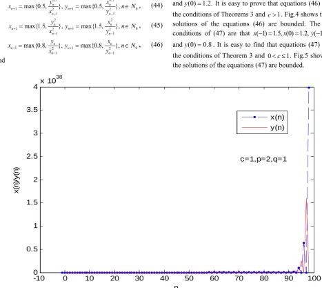
take different values, we have the followinge equations
2 2
1 1
1 1
0
}, max{1, n },
n n
n n
x max{1, yn
x y n N
x y
+ +
− −
= ∈
,
(43)=
0.5 0.5
1 2 1 2
1 1
max{0.5, n }, max{0.5, n },
n n
n n
y x
0
x y
x y
+ +
− −
= = n∈N , (44)
2 2
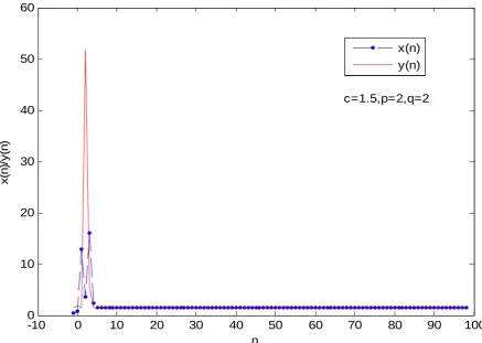
1 2 1 2
1 1
max{1.5, n }, max{1.5, n },
n n
n n
y x
0
x y
x y
+ +
− −
= = n∈N , (45)
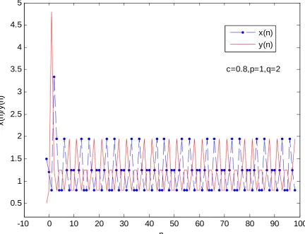
1 2 1 2
1 1
max{0.8, n}, max{0.8, n },
n n
n n
y x
0
x y
x y
+ +
− −
= = n∈N
,
(46)and
More precisely, the initial conditions of (43) are that ( 1) 0.5, (0) 0.8, ( 1) 0.8
x− = x = y − = and . It is easy
to show that the equations (43) satisfy the conditions of Theorem 1. Fig.1 shows that the solutions of the equations (43) are unbounded. The initial conditions of (44) are that
(0) 1.2
y =
( 1) 0.2, (0) 0.4, ( 1) 0.8
x− = x = y − = and It is not
difficult to find that the equations (44) satisfy the conditions of Theorem 2 and
(0) 0.7.
y =
2
p ≤q. Fig.2 shows that the solutions of
the equations (44) are bounded. The initial conditions of equations (45) are that x( 1) 0.5, (0) 0.8, ( 1) 1.2− = x = y − = and . It is obvious that equations (45) satisfy the condition of Theorems 2 and . Fig.3 shows that the solutions of the equations (45) are bounded. The initial condition of (46) is that
and
(0) 1.8
y =
2 4q p> >q
( 1) 1.2, (0) 1.4, ( 1) 1.5
x − = x = y− =
(0) 1.2.
y = It is easy to prove that equations (46) satisfy the conditions of Theorems 3 and . Fig.4 shows that the solutions of the equations (46) are bounded. The initial
conditions of (47) are that
and
1
c>
( 1) 1.5, (0) 1.2, ( 1) 0.5
x− = x = y− =
(0) 0.8
y = . It is easy to find that equations (47) satisfy the conditions of Theorem 3 and . Fig.5 shows that the solutions of the equations (47) are bounded.
0< ≤1c
-10 0 10 20 30 40 50 60 70 80 90 100
0 0.5 1 1.5 2 2.5 3 3.5
4x 10 38
n
x(
n
)/
y(
n
)
[image:4.595.54.522.327.744.2]c=1,p=2,q=1 x(n) y(n)
Fig. 1. The solutions of the equation (43) with the initial conditions x( 1) 0.5, (0) 0.8, ( 1) 0.8, (0) 1.2− = x = y− = y =
IAENG International Journal of Applied Mathematics, 46:4, IJAM_46_4_14
-10
0
10
20
30
40
50
60
70
80
90
100
0
5
10
15
20
25
n
x(
n
)/
y(
n
)
[image:5.595.80.514.50.386.2]c=0.5,p=0.5,q=2
x(n)
y(n)
Fig. 2. The solutions of the equation (44) with the initial conditionsx( 1) 0.2, (0) 0.4, ( 1) 0.8, (0) 0.7− = x = y− = y =
-10 0 10 20 30 40 50 60 70 80 90 100
0 10 20 30 40 50 60
n
x(
n
)/
y
(n
)
c=1.5,p=2,q=2 x(n) y(n)
Fig. 3. The solutions of the equation (45) with the initial conditionsx( 1) 0.5, (0) 0.8, ( 1) 1.2, (0) 1.8− = x = y − = y =
IAENG International Journal of Applied Mathematics, 46:4, IJAM_46_4_14
[image:5.595.77.515.421.732.2]-10 0 10 20 30 40 50 60 70 80 90 100 1
1.1 1.2 1.3 1.4 1.5
n
x(
n
)/
y(
n
)
[image:6.595.78.516.54.357.2]c=1.1,p=1,q=0.125 x(n) y(n)
Fig. 4. The solutions of the equation (46) with the initial conditionsx( 1) 1.2, (0) 1.4, ( 1) 1.5, (0) 1.2− = x = y − = y =
-10
0
10
20
30
40
50
60
70
80
90
100
0.5
1
1.5
2
2.5
3
3.5
4
4.5
5
n
x(
n
)/y(
n
)
c=0.8,p=1,q=2
x(n)
y(n)
Fig. 5. The solutions of the equation (47) with the initial conditionsx( 1) 1.5, (0) 1.2, ( 1) 0.5, (0) 0.8− = x = y− = y =
IAENG International Journal of Applied Mathematics, 46:4, IJAM_46_4_14
[image:6.595.81.514.395.726.2]IV CONCLUSIONS
In this paper, we have dealt with the problem of boundedness character for a class of max-type difference system. And we have obtained some sufficient conditions which ensure the boundedness character of the max-type system. The sufficient conditions that we obtained are very simple, which provide flexibility for the application and analysis of max-type difference system. These results generalize and improve some previous works. In addition, we present the use of a new iteration method for symmetric systems of max-type difference equations. This technique is a powerful tool for solving various difference equations and it can be applied to other nonlinear differential equations in mathematical physics. Computations are performed using the software package Matlab R2013b. In particular, some numerical examples are given to show the validity of the obtained theoretic results
REFERENCES
[1] Z. Yan and X. Jia, "Existence of Fractional Stochastic Schrodinger
Evolution Equations with Potential and Optimal Controls," IAENG
International Journal of Applied Mathematics, vol. 46, no.2, pp. 210
-222, 2016
[2] L. Li, and B. Du, "Global Asymptotical Stability in a Stochastic
Predator-Prey System With Variable Delays," IAENG International
Journal of Applied Mathematics, vol. 46, no.2, pp. 241-246, 2016.
[3] D. Jana and E. M. Elsayed, “Interplay between strong Allee effect,
harvesting and hydra effect of a single population discrete-time system,” International Journal of Biomathematics, vol. 9, no. 1, Article
ID 1650004, 2016.
[4] M. Kolar, M. Benes, D. Sevcovic, and J. Kratochvil, "Mathematical
Model and Computational Studies of Discrete Dislocation Dynamics,"
IAENG International Journal of Applied Mathematics, vol. 45, no.3, pp. 198-207, 2015
[5] J. E. Macias-Diaz, “A positive finite-difference model in the
computational simulation of complex biological film models,” Journal
of Difference Equations and Applications, vol. 20, no. 4, pp. 548-569,
2014.
[6] K. Anada and T. Ishiwata, "Some Features for Blow-up Solutions of a
Nonlinear Parabolic Equation," IAENG International Journal of
Applied Mathematics, vol. 45, no.3, pp. 175-182, 2015.
[7] A. Gelisken and C. Cinar, “On the global attractivity of a max-type
difference equation,”Discrete Dynamics in Nature and Society, vol.
2009, Article ID 812674, 5 pages, 2009.
[8] L. X. Hu, W. S. He, and H. M. Xia, “Global asymptotic behavior of a
rational difference equation,” Applied Mathematics and Computation,
Vol. 218, no. 15, pp. 7818-7828, 2012.
[9] E. M. Elsayed, “Behavior and Expression of the Solutions of Some
Rational Difference Equations,” Journal of Computational Analysis
and Applications, Vol. 15, pp. 73-81, 2013.
[10] E. A. Grove and G. Ladas, Periodicities in Nonlinear Difference
Equations, Chapman & Hall, CRC Press, 2005.
[11] W.T. Patula, H.D. Voulov, “On a max type recurrence relation with
periodic coefficients,” Journal of Difference Equations and
Applications, vol. 10, no. 3, pp. 329-338, 2004.
[12] E. M. Elsayed and B. D. Iricanin, “On a max-type and a min-type
difference equation,” Applied Mathematics and Computation, Vol. 215,
no. 2, pp. 608-614, 2009.
[13] Q. Xiao and Q. Shi, “Eventually periodic solutions of a max-type
equation,”Mathematical and Computer Modelling, vol. 57, no. 3-4,
pp. 992-996, 2013.
[14] S. Stević, “Some results on max-type difference equations, The
Modelling of Nonlinear Processes and Systems (International Science Conference. Book of abstracts. Moscow),” Russia, October 14-18, pp.
140, 2008.
[15] S. Stević, “On a nonlinear generalized max-type difference equation,”
Journal of Mathematical Analysis and Applications, Vol. 376, no. 1, pp.
317-328, 2011.
[16] S. Stević, “On a symmetric system of max-type difference equations,”
Applied Mathematics and Computation, Vol. 219, no. 15, pp. 8407-8412, 2013.
[17] F. Sun, “On the asymptotic behavior of a difference equation with
maximum,” Discrete Dynamics in Nature and Society, Vol. 2008,
Article ID 243291, 6 pages, 2008.
[18] A. Gelisken and C. Cinar, “On the global attractivity of a max-type
difference equation,”Discrete Dynamics in Nature and Society, vol.
2009, Article ID 812674, 5 pages, 2009.
[19] T. F. Ibrahim and N. Touafek, “Max-type system of difference
equations with positive two-periodic sequences,” Mathematical
Methods in the Applied Sciences, Vol. 37, no. 16, pp. 2541-2553, 2014.
[20] M. M. El-Dessoky, “On the periodicity of solutions of max-type
difference equation,” Mathematical Methods in the Applied Sciences,
Vol. 38, no. 15, pp. 3295-3307, 2015.