Accurate Reconstruction of Discontinuous
Functions Using the Singular Padé-Chebyshev
Method
Arnel L. Tampos, Jose Ernie C. Lope and Jan S. Hesthaven
Abstract— In this paper, we present a singularity-based resolution of the Gibbs phenomenon that obstructs the recon-struction of a function with jump discontinuities by a truncated Chebyshev series or a Padé-Chebyshev approximation. We tackle the more difficult case where the jump locations are not known. The identification of unknown singularities is carried out using a Padé-Chebyshev approximation. Numerical examples to illustrate the method are provided, including an application on postprocessing computational data corrupted by the Gibbs phenomenon.
Index Terms— Gibbs phenomenon, function reconstruction, Padé-Chebyshev approximation
I. INTRODUCTION
Approximation of smooth functions by Fourier series or by truncated orthogonal polynomial expansions in general is known to be exponentially convergent and highly accurate ([2], [6]). For functions with singularities, however, con-vergence of a partial sum of orthogonal series is adversely affected in the area over which the singularities occur, a prob-lem which has come to be known as the Gibbs phenomenon. This phenomenon manifests in an oscillatory behavior at the vicinity of the jumps and thus presents an obstruction in the reconstruction of a discontinuous function.
An exposition on the nature of the Gibbs phenomenon and some remediation schemes to counter its effect can be found in [5], [7], and [8]. A class of techniques aimed at resolving the Gibbs phenomenon comprises Padé-type approximations (e.g. [1], [2], [3], [7], [9], [12]). These methods extend the standard Padé approximation by making use of orthogonal polynomials as basis in lieu of the canonical basis with which the numerator and denominator of a Padé approximant are expanded. A Padé-type approximant enjoys the advantage of utilizing rational functions, which are broader than polyno-mials and can have singularities, and hence there is a stronger likelihood that it will capture the singularities of the function being approximated ([2], [7]).
Some Padé-based methods work without requiring infor-mation about the jump locations. However, locating jump discontinuities can become a relevant issue when the actual function is not explicitly known. In many cases, for instance, involving spectral approximations of nonsmooth solutions to some partial differential equations, the solution comes in the
Arnel L. Tampos is with the Division of Physical Sciences and Mathe-matics, University of the Philippines Visayas, Miag-ao, Iloilo, Philippines. Email: [email protected]
Jose Ernie C. Lope is with the Institute of Mathematics, Uni-versity of the Philippines Diliman, Quezon City, Philippines. Email: [email protected]
Jan S. Hesthaven is with the Division of Applied Mathematics, Brown University, Providence, R.I., USA. Email: [email protected]
form of computational data that are contaminated by Gibbs phenomenon. As these data are noisy, the standard procedure is to postprocess them to correct the phenomenon. One way this can be done, as demonstrated in [1], [7], and [14], is to use Padé-type approximation. This Padé postprocessing approach, however, may turn out to be less successful unless fed with some information about the possible jump positions which, as noted in [7], can be advantageous for its effective implementation. As computational data may not show explicitly the existence and whereabouts of possible jumps, to somehow locate them can become imperative.
A study by Driscoll and Fornberg ([2], [3]) reveals just how significant the knowledge of the jump locations can be in correcting the Gibbs phenomenon. Realizing that the poles available in a rational approximant do not intrinsically and adequately reproduce the jump behaviors of a discontinuous function f, they devised an approach that incorporates the jump locations into the approximation process. A similar approach that imbibes this concept in the context of Padé-Chebyshev approximation is discussed in [12]-[14].
This paper is anchored on the Singular Padé -Chebyshev (SPC) approximation introduced in [12] and further dis-cussed in [13] and [14], a brief review of which is presented in the next section. Section 3 discusses a Padé-based ap-proach in identifying singularities of the function. Section 4 focuses on some numerical results of the SPC implementa-tion in reconstructing some test funcimplementa-tions and postprocessing computational data contaminated by the Gibbs phenomenon.
II. A SINGULARITY-BASEDPADÉ-CHEBYSHEV
APPROXIMATION
For a function f : [−1,1] → R belonging to L2
ω space with Chebyshev weight function ω, the Chebyshev series expansion T(f)off is defined by
T(f) =
∞
X
n=0
cnTn, cn=
hf, TniL2
ω kTnk2L2
ω
, (1)
where the Tns are the Chebyshev polynomials of the first kind defined as Tn(x) = cos (nθ),θ= cos−1(x),
hf, TniL2
ω =
ˆ 1
−1
f(x)Tn(x) 1
√
1−x2dx
and
kTkkL2
ω=
(√
π, n= 0
pπ
2, n≥1.
Alternatively, we may express (1) as
f(x) =c0 2 +
∞
X
n=1
cnTn(x), (2)
IAENG International Journal of Applied Mathematics, 42:4, IJAM_42_4_07
with cn =
2 π
ˆ 1
−1
f(x)Tn(x)
√
1−x2 dx, n= 0,1,2, . . . . (3)
The coefficientscnmay be approximated using the following Gauss-Chebyshev quadrature rule
ˆ 1
−1
h(x)ω(x)dx∼= m
X
k=1
Akh(xk), (4)
where {xk} are the zeros of the Chebyshev polynomials Tm(x) = cos (mθ), h(x) = f(x)Tn(x), ω(x) = √11−x2, andAk =mπ for allk.
By the definition of Tn and the fact that cos(nθ) =
1 2 e
inθ+e−inθ
, we can introduce the variablez=eiθ and transform (2) into
f(z) =1 2
∞ X0
n=0
cnzn+
∞
X0
n=0 cnz−n
,
where the primed sum indicates that the first term in the summation is halved. Let
g(z) =
∞
X0
k=0
cnzn. (5)
Then (2) becomes f(z) =1
2 g(z) +g z
−1
.
We refer tog(z)as thetransformed Chebyshev series asso-ciated with f(z), and consequently with f(x). As f(x) =
<[g(z)], with <[·] denoting the real part of the function, approximatingf is tantamount to approximatingg(z). Thus, truncating the series g(z) up to degree N determines a Chebyshev approximant to f of order N and we denote this orthogonal polynomial approximant by Cheb(N). As pointed earlier, approximating a discontinuous function by a truncated orthogonal series such as Cheb(N) suffers from the Gibbs phenomenon, a problem which may be circum-vented using some Padé-based techniques.
For a piecewise analytic function f defined on [−1,1] with associated transformed Chebyshev seriesg(z), its Padé-Chebyshev approximant of order(N, M)can be defined by the rational function
R(N,M)(z) = PN(z) QM(z)
= N
X
k=0 pkzk
M
X
k=0 qkzk
, (6)
wherez =eicos−1(x) andQM is not identically zero, such that
QM(z)g(z)−PN(z) =O zN+M+1
, z→0.
We denote the approximant defined in (6) byP C(N, M). A drawback in a Padé-type approximant such as (6), as observed in the case of the Fourier-Padé approximation ([2], [3]), lies in its inability to sufficiently resolve the Gibbs phenomenon. Driscoll and Fornberg discussed in [2] and [3] a Padé-based correction of this phenomenon that takes into account the singularities of the function. Applying their argument in our context, a jump discontinuity of a function
at a point x=ξ can be incorporated into the seriesg(z)by a logarithm term which takes the form of
log1− z
eiθξ
, (7)
where0≤θξ = cos−1(ξ)≤π. This logarithmic singularity is utilized to redefine (6) in the same way as it is handled in [2] and [3].
Let f(x) be a piecewise analytic function defined on [−1,1] with s jump locations at x = ξk ∈ [−1,1], k = 1, . . . , s, and consider its associated transformed Chebyshev series (5). In view of (7), the Padé-Chebyshev approximant (6) may now be modified as
R(z) =
PN(z) + s
X
k=1
RVk(z) log
1− z
eiθk
QM(z)
, (8)
wherez=eicos−1(x) and
PN(z) = N
X
j=0
pjzj, QM(z) = M
X
j=0
qjzj 6= 0,
RVk(z) =
Vk
X
j=0
r(jk)zj, k= 1, . . . , s,
such that
QM(z)g(z)−[PN(z) +U(z)] =O zη+1
,
with
U(z) = s
X
k=1
RVk(z) log
1− z
eiθk
and
η=N+M+s+ s
X
k=1 Vk.
The function in (8) defines the Singularity-based Padé-Chebyshev (SPC) approximant to f of order (N, M, V1, . . . , Vs) and we denote this approximant
by SP C(N, M, V1, . . . , Vs).
Proposition 1. The approximant defined in (8) exists and is unique.
Proof: (See [12].)
The unknown coefficients of polynomials PN, QM, and RVks are then computed through the following linear system
of η+ 1 equations inη+ 2variables: M
X∗
j=0
cN−j+tqj− V1
X
j=0
a(1)N−j+tr(1)j −· · ·−
Vs
X
j=0
a(Ns)−j+tr(js)= 0,
M
X∗
j=0
cl−jqj− V1
X
j=0
a(1)l−jrj(1)− · · · −
Vs
X
j=0
a(ls−)jr(js)=pl,
where t = 1, . . . , η−N, l = 0, . . . , N, and the asterisk-marked summation indicates that the term withc0 is halved.
We note that in this system, cn = 0, for n <0. It should be noted too that the a(nk) are the coefficients in the Taylor expansion of
log1− z
eiθk
= ∞ X n=1 − 1
neinθk
zn
IAENG International Journal of Applied Mathematics, 42:4, IJAM_42_4_07
and a(nk) = 0, for n ≤ 0. Accordingly, R(z) defined by (8) approximatesg(z)which implies that the real part ofR
approximatesf(x).
Proposition 2. For the SPC approximant defined in (8), we have
|f(z)− <(R(z))| ≤ 1 |QM(z)|
X
l>η
|bl|
wherez=eicos−1(x),η=N+M+s+ s
X
k=1 Vk, and
bl= M
X∗
j=0
cl−jqj− V1
X
j=0
a(1)l−jrj(1)− · · · −
Vs
X
j=0
a(l−s)jr(js),
a(nk) being the coefficients in the Taylor expansion of log 1− z
eiθk
, cn = 0, for n < 0 , and ,a
(k)
n = 0 for n≤0.
Proof: (See [12].)
III. APPROXIMATEJUMPLOCATIONS OF A
DISCONTINUOUSFUNCTION
There have been studies on locating jump discontinuities of a discontinuous function ([3], [4], [7]) and some of these explore the connection between jump locations and the differentiated series expansion of the function. Estimating jump locations using Padé approximation is introduced in [3] and its applicability is based on the idea that a Padé approximation of the differentiated series expansion of a discontinuous function f likely leads to an ordinary pole at a jump location. As our approach is founded on Padé-Chebyshev approximation, we further pursue this idea to gen-erate information about the jump locations of discontinuous functions.
For the derivative off, a Padé-Chebyshev approximant of order(N, M)may be defined as
Rf0(z) =
(Pf0)
N(z) (Qf0)
M(z)
, (9)
wherez=eicos−1(x) and
(Pf0)
N(z) = N
X
j=0
(pf0)
jz j,
(Qf0)
M(z) = M
X
j=0
(qf0)
jz j 6= 0,
such that (Qf0)
M(z)g
0(z)−(P
f0)
N(z) =O z
N+M+1
.
Finding the unknown coefficients of polynomials(Pf0)
N and (Qf0)
M is tantamount to solving the following linear system:
M X j=0
i(N+λ−j+ 1)cN+λ−j+1(qf0)
j= 0,
λ= 0,1,2, . . . , M−1, M
X
j=0
i(µ−j)cµ−j(qf0)
j = (pf0)µ,
µ= 1,2. . . , N,
where i= √−1 and the expansion coefficients ck = 0for each k <0. We remark thatRf0 is a Padé-Chebyshev (PC)
approximant that approximates g0(z)which is the derivative
of the transformed Chebyshev series associated with f(x). Consequently, the real part of Rf0 approximatesf0(x).
Recalling the definition of the Chebyshev polynomial, we know thatθ= cos−1(x)withx∈[−1,1]andθ∈[0, π]. This defines a mapping from[−1,1]onto[0, π]. The transforma-tion z = eiθ consequently maps [−1,1] to the upper half of the unit circle in the complex plane at which eiθ
= 1.
Now consider the Padé-Chebyshev approximant Rf0 to g0.
Let z0 be a zero of (Qf0)
M or a pole of Rf0. We have
z0 = eiθ0 for some θ0 ∈ [0, π]. By the inverse mapping, |z0|= 1implies thatz0corresponds to a pointx0in[−1,1].
Asz0is a singularity,x0 must be a jump off(x)in[−1,1].
Furthermore, since z0= cosθ0+isinθ0, the jump must be
located at x0 = cosθ0 =<(z0). The preceding discussion
is summarized in the following proposition.
Proposition 3. A pole z0 of Rf0 for which |z0| = 1
corresponds to a jump discontinuity off(x)in[−1,1]which occurs atx=<(z0).
This provides a simple criterion by which we may be able to locate a jump discontinuity of a piecewise contin-uous function using the Padé-Chebyshev approximant of its differentiated series expansion. As stated, we only need to consider those zeros of (Qf0)
M for which the modulus is equal to (or approximately) 1 in order to identify the zeroth-order jumps of the function.
The result of this section can be extended naturally to allow the identification of a first-order jump in a continuous function with discontinuous first derivative and also higher-order jumps for functions belonging to class Ck[−1,1]ofk times continuously differentiable functions.
IV. NUMERICALRESULTS
The SPC method applied to classical test functions such as the signum function and the absolute value functionf(x) =
|x| effectively resolves the Gibbs phenomenon present in both the Cheb(N) and P C(N, M) approximants of these functions (see [12] and [13]). In this section, we continue to demonstrate the efficacy of the method by reconstructing the following piecewise smooth functions:
1) f1(x) =
√
1−x2, 0≤x≤1
0, −1/2≤x <0
−x−1, −1≤x <−1/2
2) f2(x) =
−2 sin−1x, −1≤x <−2 3
exp −x2
+x, −2
3 ≤x <0.2
cos(3πx) + 2x, 0.2≤x≤1.
We then show how the method recovers a function from a computational data set that is contaminated by the Gibbs phenomenon. In this regard, we consider reconstructing a function that is given in terms of computational data from the numerical solution to the following viscous Burgers’ equation:
∂u ∂t +u
∂u ∂x =
∂2u
∂x2, x∈[−1,1], = 0.001 (10)
IAENG International Journal of Applied Mathematics, 42:4, IJAM_42_4_07
with boundary conditions
u(−1, t) =u(1, t) = 0 (11) and initial condition
u(x,0) =−tanh
x+ 0.5
2
+ 1. (12)
The numerical implementation for function reconstruction was done in Scilab, an open-source software.
A. Reconstructingf1
By definition,f1has discontinuities atx= 0andx=−12.
With reference to Table I, it is interesting to note that the approximate locations of these jumps may be obtained using (9) and Proposition 3.
Table I ZEROS OFQf0
1OF THEP C(15,15)APPROXIMANT AND THE
APPROXIMATE JUMP LOCATIONS OFf1. (*INDICATES NO RELATION WITH THE JUMP.)
Approximating Jump Locations off1
Zeros ofQf0
1 Modulus Jump at
−0.50105±0.86647i 1.00091 x≈ −0.5 −0.00012±1.00007i 1.00007 x≈0 −0.49876±1.00989i 1.12634 *
−0.31860±1.45791i 1.49231 *
0.77977±2.78340i 2.89057 *
0.88246 0.88246 *
1.03498 1.03498 *
1.20644 1.20644 *
1.76114 1.76114 *
362.86831 362.86831 *
The exact Chebyshev coefficients in the Chebyshev ex-pansion of f1 are given by
cn=
−2 3+
2+√3
π , n= 0
1+√3
π −
√ 3 4π −
1
3, n= 1
k, n≥2,
where
k = 2nsin nπ
2 −nsin 2nπ3 −
√
3 cos 2nπ3 −2
n2−1
π
+ 2 nπsin
2nπ 3 .
The SPC approximant for f1 is determined by P(z) +R1(z)L1(z) +R2(z)L2(z)
Q(z) ,
where
L1(z) = log
1−z
i
and
L2(z) = log
"
1− z
exp 2πi3
#
.
Figure 1 shows the Gibbs phenomenon in a PC approxi-mation of f1. The oscillation caused by the phenomenon is
[image:4.595.316.524.72.226.2]practically eliminated upon the inclusion of the function’s singularities into the approximation process as shown in Figure 2. An SPC approximant of f is shown in Figure 2 against the graph of the exact function. The reconstruction is remarkably good that the graph of the exact function is hardly
[image:4.595.75.263.299.419.2]Fig. 1. Contrast between the exactf1and its PC(15,12) approximant.
Fig. 2. Contrast between the exactf1 and its SPC(15,12,10,10)
approxi-mant.
noticeable. As shown in Figure 3, this impressive result by the SPC approximation is clearly marked by an improved convergence of the pointwise error.
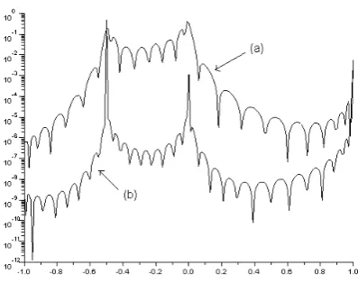
Fig. 3. Comparison of the pointwise error convergence in logarithmic scale of (a) PC(15,12) and (b) SPC(15,12,10,10) approximants off1.
IAENG International Journal of Applied Mathematics, 42:4, IJAM_42_4_07
[image:4.595.44.274.461.705.2] [image:4.595.321.520.594.751.2]B. Reconstructingf2
The function f2 is a test function with a somewhat
[image:5.595.323.524.75.225.2]com-plicated shape. It is discontinuous atx= 0.2 andx=−2 3.
[image:5.595.82.258.175.257.2] [image:5.595.320.522.283.434.2]Table II gives information about approximate locations of these singularities obtained using (9) and Proposition 3.
Table II ZEROS OFQf0
2OF THEPC(20,10)APPROXIMANT AND THE
APPROXIMATE JUMP LOCATIONS OFf2.
Approximating Jump Locations off2
Zeros ofQf0
2 Modulus Jump at
−0.65871±0.75255i 1.00012 x≈ −2/3
0.19454±0.99007i 1.00900 x≈0.2 0.29769±1.14446i 1.18254 *
0.73156±1.63159i 1.78809 *
0.00776 0.00776 *
−1.04728 1.04728 *
The exact Chebyshev coefficients in the Chebyshev ex-pansion of f2 are given by
cn=C1+C2+C3,
where
C1 =
ˆ π
cos−1(−2 3)
−2 sin−1(cosθ) cosnθdθ,
C2 =
ˆ cos−1(−2 3)
cos−1(0.2)
exp −cos2θ
+ cosθ
cosnθdθ,
C3 =
ˆ cos−1(0.2)
0
[cos (3πcosθ) + 2 cosθ] cosnθdθ.
Using (4), these coefficients are approximated as
g(xk) =
B1, −1≤x≤ −23 B2, −23 ≤x <0.2,
B3, 0.2≤x <1
(13)
where
B1 = −2 sin−1(xk) cos
ncos−1(xk)
B2 = exp−cos2(xk)+xk cosncos−1(xk) B3 = [cos (3πxk) + 2xk] cos
ncos−1(xk)
.
The SPC approximant off2 is given by P(z) +R1(z)L1(z) +R2(z)L2(z)
Q(z) ,
where
L1(z) = log
(
1− z
exp
icos−1(−2/3) )
,
and
L2(z) = log
(
1− z
exp
icos−1(0.2) )
.
Fig. 4. The Gibbs phenomenon in the Cheb(126) approximant off2.
Fig. 5. A resolution of the Gibbs phenomenon by the SPC(126,10,8,3) approximant off2, shown here against the exact function.
Fig. 6. Comparison of the pointwise error convergence in logarithmic scale of (a) Cheb(126) and (b) SPC(126,10,8,3) approximants off2.
In lieu of the exact form, the approximated Chebyshev coefficients (13) are used in the reconstruction of the func-tion. Using250Gauss-Chebyshev quadrature points, the SPC (126,10,8,3) approximant for f2, shown in Figure 5, almost
smoothens the Gibbs phenomenon (Figure 4) seen in the polynomial approximation of the function by Cheb (126).
IAENG International Journal of Applied Mathematics, 42:4, IJAM_42_4_07
[image:5.595.47.283.315.445.2] [image:5.595.317.520.514.668.2]The pointwise errors shown in Figure 6 demonstrate that the reconstruction is practically good.
C. Recovering Solution to Burger’s Equation
Numerical solution to the Burgers’ equation by spectral method generates a set of computational data that is cor-rupted by the Gibbs phenomenon in the sense that solutions to such equation are known to develop sharp gradient in time [1]. Here we present some results on the use of the SPC ap-proximation to postprocess or “clean up” the data inorder to recover the solution to the viscous Burger’s equation defined in (10)-(12). This equation is a suitable model for testing computational algorithms for flows where steep gradients or shocks are anticipated because it allows exact solutions for many combinations of initial and boundary conditions [1]. It should be noted that the postprocessing needs only to be applied at time levels at which a “clean” solution is desired, and not at every time step [11].
In this case, the transformed Chebyshev series for the solution assumes expansion coefficients that are approxi-mated using (4). The input data are given at 100 Gauss-Chebyshev quadrature points. Working on the assumption that there may be some inherent jump discontinuities or sharp gradient not known or readily observable from the data, we first seek the locations of these possible jumps or shocks in the data by way of the Padé approximation applied to the differentiated expansion that represents the solution u. Incorporating the resulting shock information into the SPC approximation generates a reconstructed u. For illustration, let us consider the case when time t = 0 and t = 0.1. Under each case, we take as inputs some computed data that serve as values ofuat the given Gauss-Chebyshev quadrature points.
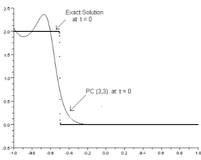
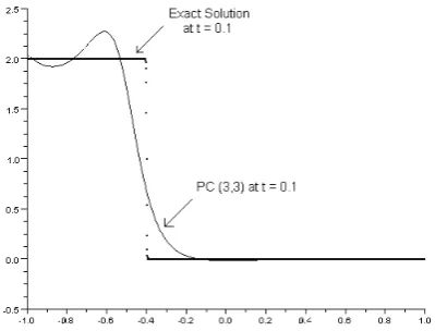
Determined by the PC(3,3) approximant to the differenti-ated transformed Chebyshev expansion associdifferenti-ated with u, Figure 7 shows that at t = 0 a possible jump or shock occurs somewhere very close to x = −0.5. The zeros of the denominator of the PC(3,3) approximant are −0.00764 and−0.49321±0.86966i. The complex zero gives a modulus of 0.99978 which strongly indicates that a shock occurs at x=−0.49321. This confirms what the plot shows. For the case when t= 0.1, Figure 8 indicates that there is a shock very near x =−0.4. The zeros of the denominator of the PC(3,3) approximant in this case are −0.40666±0.91406i and−1.61685. The complex zero gives a modulus of 1.00043 implying that a shock location is atx=−0.40666, which is what the plot seems to suggest. In consideration of the two different shock positions at two different points in time, we note that the Burgers’ solution involves time evolution of a shock or a sharp gradient.
[image:6.595.319.521.73.225.2]We present the PC(3,3) and SPC(3,3,3) reconstructions of uin Figures 9 and 11 for the caset= 0and in Figures 10 and 12 for t= 0.1. They are plotted against the exact solution. Both approximants in the two cases take the PC approxi-mated jump locations, that is, the jump at x = −0.49321 for t = 0 and the jump at x = −0.40666 for t = 0.1. The SPC results are quite impressive notwithstanding the fact the we only use low order approximants to generate them. Comparisons of their respective pointwise error convergence are shown in Figures 13 and 14.
[image:6.595.318.523.305.470.2]Fig. 7. Approximate shock location ofuatx= – 0.49321 when t= 0, using PC(3,3) approximant foru0.
[image:6.595.321.520.562.720.2]Fig. 8. Approximate shock location ofuatx= – 0.40666 whent= 0.1, using PC(3,3) approximant foru0.
Fig. 9. Contrast between the exact solution and its PC(3,3) approximant att= 0.
IAENG International Journal of Applied Mathematics, 42:4, IJAM_42_4_07
Fig. 10. Contrast between the exact solution and its PC(3,3) approximant att= 0.1.
Fig. 11. Contrast between the exact solution and its SPC(3,3,3) approxi-mant att= 0.
[image:7.595.320.521.301.455.2]Fig. 12. Contrast between the exact solution and its SPC(3,3,3) approxi-mant att= 0.1.
Fig. 13. Comparison of the pointwise error convergence in logarithmic scale of (a) PC(3,3) and (b) SPC(3,3,3) approximants oft= 0.
Fig. 14. Comparison of the pointwise error convergence in logarithmic scale of (a) PC(3,3) and (b) SPC(3,3,3) approximants oft= 0.1.
D. Some Remarks on the Degrees ofPN,QM, and theRVks
that Define the SPC Approximant
In the course of implementing the SPC method, choosing the degrees of the polynomials PN, QM, and RVks that
comprise the SPC approximant can be a crucial issue. In the absence of a rigorous and optimal means of generating these values ([2], [7]), one is left to try several possible combinations. While certain combinations are good which lead to fairly accurate reconstructions, some are obviously bad which either do not remove oscillations or may smoothen out some part but add extraneous oscillations and jumps at the other or cause the jump(s) to steepen further. A simple rule is to compute many approximants with various combinations, select those that are reasonably good, and disregard the bad recontructions [7]; generating an SPC approximant is quick and easy, afterall.
V. CONCLUSION
The Singular Padé-Chebyshev (SPC) approximation demonstrates howP C(N, M)andCheb(N)reconstructions of a function with singularities can be enhanced by utilizing its singularities in the approximation process. If the singular-ities are known, the SP C(N, M, V1, . . . , Vk) approximant
IAENG International Journal of Applied Mathematics, 42:4, IJAM_42_4_07
[image:7.595.63.268.308.485.2] [image:7.595.64.266.587.753.2]remarkably reconstructs such function. Under restrictive con-ditions where only the approximated expansion coefficients for the transformed Chebyshev series of the function and the approximated jump locations are used, as in the case of postprocessing computational data, numerical results still reveal that SPC approximant is capable of rectifying the Gibbs phenomenon that occurs in the process of recovering the function. A study on best combinations of the degreesN, M,V1, ...,Vk in the SPC approximants that yield excellent reconstructions may be pursued as this may not only promote greater ease in approximation but will pave the way as well for a systematic construction of the approximant.
REFERENCES
[1] W. S. Don, S. M. Kaber, and M. S. Min, “Fourier-Padé approximations and filtering for the spectral simulations of incompressible Boussinesq convection problem,”Math. Comp., 76 (2007), pp. 1275-1290. [2] T. A. Driscoll and B. Fornberg, “A Pade-based algorithm for
over-coming the Gibbs phenomenon,”Numer. Algorithms, 26 (2001), no.1, pp.77 - 92
[3] T. A. Driscoll and B. Fornberg. “Pade-based interpretation and cor-rection of the Gibbs phenomenon,” InAdvances in the Gibbs
Phe-nomenon, ed. by A. Jerri, Sigma Sampling Publishing, Potsdam, NY,
2007.
[4] A. Gelb and E. Tadmor, “Detection of edges in spectral data,”Appl.
Comput. Harmon. Anal., 7 (1999), pp. 101–135.
[5] D. Gottlieb and C. W. Shu, “On the Gibbs phenomenon and its resolution,”SIAM Rev., 39 (1997), pp. 644-668.
[6] J. S. Hesthaven, S. Gottlieb, D. Gottlieb,Spectral Methods for
Time-Dependent Problems, Cambridge University Press, U.K., 2007
[7] J. S. Hesthaven, S. M. Kaber, L. Lurati, “Padé-Legendre interpolants for Gibbs reconstruction,”J. Sci. Comput., 28 (2006), pp. 337-359. [8] A. J. Jerri,The Gibbs Phenomenon in Fourier Analysis, Splines and
Wavelet Approximation, Kluwer Dordrecht, 1998
[9] S. M. Kaber and Y. Maday, “Analysis of some Padé-Chebyshev approximants,”SIAM J. Numer. Anal., 43 (2005) no.1, pp. 437-454. [10] G. K. Kvernadze, “Approximating the jump discontinuities of a
function by its Fourier-Jacobi coefficients,”Math. Comp., 73 (2003), pp. 731 – 751.
[11] S. A. Sarra, S.A., “Spectral methods with postprocessing for numerical hyperbolic heat transfer,” Numer. Heat Transfer, Part A, 43, no.7 (2003), pp.717-730
[12] A. L. Tampos and J. E. C. Lope, “Overcoming Gibbs phenomenon in a Padé-Chebyshev approximation,”Matimyas Matimatika:
Proceed-ings of the 7th Taiwan-Philippine Symposium in Mathematics, 25-27
October, 2007, Antipolo, Rizal, Phil., pp.127-135.
[13] A. L. Tampos and J. E. C. Lope, “A Padé-Chebyshev Reconstruction of functions with jump discontinuities,”Lecture Notes in Engineering and Computer Science: Proceedings of the World Congress on Engineering
2009, WCE 2009, 1 - 3 July, 2009, London, U.K., pp. 1174-1179.
[14] A. L. Tampos, J. E. C. Lope, and J. S. Hesthaven, “A Singularity-based approach in a Padé-Chebyshev resolution of the Gibbs phenomenon,”
Lecture Notes in Engineering and Computer Science: Proceedings of
the World Congress on Engineering 2012, WCE 2012, 4 - 6 July, 2012,
London, U.K., pp. 24-29.