Snake Energy Analysis and Result Validation for a Mobile Laser Scanning Data Based Automated Road Edge Extraction Algorithm

Snake Energy Analysis and Results Validation for a Mobile

Laser Scanning Data based Automated Road Edge Extraction

Algorithm

Pankaj Kumar, Paul Lewis, Conor P. McElhinney, Pawel Boguslawski, Tim McCarthy

Abstract—The negative impact of road accidents can not be ignored in terms of the very sizeable social and economic loss. Road infrastructure has been identified as one of the main causes of the road accidents. They are required to be recorded, located, measured and classified in order to schedule maintenance and identify the possible risk elements of the road. Towards this an accurate knowledge of the road edges increases the reliability and precision of extracting other road features. We have developed an automated algorithm for extracting road edges from Mobile Laser Scanning (MLS) data based on the parametric active contour or snake model. The algorithm involves several internal and external energy parameters which need to be analysed in order to find their optimal values. In this paper, we present a detailed analysis of the snake energy parameters involved in our road edge extraction algorithm. Their optimal values enable us to automate the process of extracting edges from MLS data for tested road sections. We present a modified external energy in our algorithm and demonstrate its utility for extracting road edges from low and non-uniform point density datasets. A novel validation approach is presented which provides a qualitative assessment of the extracted road edges based on direct comparisons with reference road edges. This approach provides an alternative to traditional road edge validation methodologies which are based on creating buffer zones around reference road edges and then computing quality measure values for the extracted edges. We tested our road edge extraction algorithm on datasets which were acquired using multiple MLS systems along various complex road sections. The successful extraction of road edges from these datasets validates the robustness of our algorithm for use in complex route corridor environments.

Index Terms—Road Edges; Mobile Laser Scanning; Snake Energy; Validation Approach; Complex Road.

I. INTRODUCTION

Road accidents have become one of the main concerns for policy makers and road infrastructure developers due to thousands of deaths and the economic loss caused by them. Each year, around 1.24 million people die in road crashes around the world while another 20 to 50 million are severely injured [1]. Furthermore, these accidents cost between 1% and 2% of a country’s annual Gross National Product (GNP). According to the World Health Organisation (WHO) report, road traffic accidents are likely to become the fifth leading cause of death in the world by 2030 [1]. The main challenge for policy makers is to ensure that road networks are as safe as possible whilst maintaining quality and mobility.

Recent research investigations have described a significant corre-lation between road infrastructure and accident analysis values [2]. Road design has an immediate effect on accident risk as it influences driver behaviour in terms of speed, acceleration and lateral position. Road user safety may be affected by road geometry and physical features along the route corridor. These factors are required to be recorded, located, measured and classified in a timely, cost effective

P. Kumar is with the Department of Geoinformation, Universiti Teknologi Malaysia, Johor, Malaysia. E-mail: [email protected]

P. Lewis, C.P. McElhinney and T. McCarthy are with the National Cen-tre for Geocomputation, National University of Ireland Maynooth. E-mail: [email protected], [email protected], [email protected].

P. Boguslawski is with the Department of Architecture and the Built Environment, University of the West of England, Bristol, UK. E-mail: [email protected]

manner in order to schedule maintenance and ensure maximum safety conditions for road users. Safe road-way infrastructure has an important role in reducing the accident risk as it contributes to one out of three fatal accidents [3]. Road safety considerations must result in a road environment that should be self-explaining and forgiving, in the sense that users are not faced with unexpected situations and their mistakes can be, if not avoided, corrected [4].

Accurate information about the road and its features is essential for effective management of road networks and to ensure maximum safe driving conditions for road users. This information can assist decision makers to identify the possible risk elements of the road which may present a safety concern for the driving conditions. With the potential of Geographic Information Science (GIS) technologies in road management, Mobile Laser Scanning (MLS) systems present a rapid, reliable and cost effective tool for carrying out inspections along the route corridor. The European Road Safety Inspection (EuRSI) research project demonstrated that mobile mapping systems could be used to collect physical route corridor information for rapid safety analysis [5].

Mobile laser scanning systems can be employed to capture 3D spatially referenced information about the road and its surrounding environment. The use of Light Detection And Ranging (LiDAR) technology for mapping route corridors enables accurate acquisition of dense 3D point cloud data which contain elevation, intensity, pulse width, range and multiple echo attributes. These data attributes can be used for reliable and precise extraction of different road features. The road edge is a fundamental feature and its correct identification is a prerequisite in order to obtain precise information about road geometry and physical road objects. We have developed an automated algorithm for extracting road edges from MLS data [6]. This algorithm is based on a novel combination of two modified versions of the parametric active contour or snake model. In the parametric model, the snake is represented explicitly as a controlled spline curve, which is implemented based on computed energy [7]. It is defined within a 2D image domain that moves towards a desired object boundary under the influence of an internal energy within the curve itself and an external energy derived from the image data. The internal enegy is applied to the snake curve which controls the curve’s elasticity and rigidity, while the external energy attracts the snake curve towards the object boundary. The movement of the snake curve is controlled through balancing the internal and external energy terms until an energy minimisation condition is met. When the snake’s energy function reaches a minimum, it converges to the object boundary [8]. We used the parametric active contour model in our algorithm since its implementation is less computationally expensive when compared to geometric active contour models. In the geometric model, the curve is represented implicitly as a level-set and is evolved based on geometric computations, with its speed locally dependent on the image data [9,10].

In this paper, we present a detailed investigation of these parameters based on assessing the internal and external energy properties of the snake curve. We have investigated how low and non-uniform point density affects the performace of extracting features from LiDAR dataset. This was achieved by adding a modified balloon external energy in our algorithm and we demonstrate how its modified version can be useful in cases where datasets have a low and non-uniform point density along the road section. The majority of the road edge validation approaches are based on computing quality measure values with respect to the buffer zones created around reference road edges. We present a more efficient and automated approach for validating the extracted road edges based on their direct comparison with reference road edges.

In Section II, we review various methods which have been de-veloped for extracting roads and its boundaries from LiDAR data. We present a detailed review of the validation approaches which have been used to verify the extracted road boundaries. Following the review, we list the limitations in current road extraction and their validation approaches, which have been addressed through our research work. In Section III, we provide a brief description of our road edge extraction algorithm. In SectionIV, we present a detailed experimental analysis of the internal and external energy parameters involved in our algorithm. In Section V, we present the modified balloon external energy component in our algorithm. In SectionVI, we present an automated approach for validating the road edges extracted from MLS data. In SectionVII, we test our algorithm on the datasets acquired using multiple MLS systems along a variety of road sections. These test road sections consisted of distinct sets of edges, roundabout and high degree of curvature datasets. In Section

VIII, we validate the extracted road edges and discuss the test results. Finally, we conclude our paper in SectionIX.

II. LITERATUREREVIEW

MLS system provides 3D point cloud data which can be useful for extracting road features. Most methods developed for extracting road features are based on identification of planar or smooth surfaces and the classification of point cloud data on the basis of its attributes [11]. A robust evaluation of the extracted road features is also important for assessing the relevance of method for practical applications [12]. Elberink and Vosselman [13] reconstructed 3D road models by assigning airborne LiDAR points to 2D topographic map polygons. The height values of map points were calculated by fitting a least square plane to the LiDAR points inside the polygon. The precision of map point heights was calculated from error propagation based on laser point noise, systematic laser data errors and plane fitting uncertainty components. The quality of reconstructed 3D model was estimated against the photogrammetric derived topographic database [14]. Jaakkola et al. [15] delineated road kerb by filtering the gradient image of elevation information obtained from MLS system. Their evaluation approach was based on calculating completeness, correctness and mean accuracy values against manual classification of the dataset. Goepfert and Rottensteiner [16] applied the snake model to extract road network from airborne LiDAR data. In their approach, the snake curve was initialised near the road feature using available vector data while the external energy terms were derived from elevation, intensity and surface roughness information obtained from the LiDAR points. The orthophotos were manually digitised to create reliable reference data for validation purpose. The extracted road network was validated by finding a mean point to contour distance between the reference and the final position of the snake curve. Boyko and Funkhouser [17] presented a method for extracting urban roads from a large scale mobile and aerial laser scanning datasets. An initial approximation of the road network in the point

cloud was made using 2D map while the elevation based attractor function was used as an external energy of the snake to find the road edges. The road detection results were evaluated by comparing them with a manually created 2D road grid. The LiDAR points predicted as road were projected into the 2D grid and then the value of each grid cell was set to 1 if it contains the point, otherwise 0. These values were used to compute the accuracy metrics such as correctness, completeness, quality, average spill size and direction, where spill represents the distance of the extracted road side from the manually extracted road side. Ibrahim and Lichti [18] extracted street kerb and its surface by applying the derivate of gaussian function to the ground segment refined from MLS data.The extracted kerbs were evaluated by measuring its distance from manually extracted kerb at each point. The K-D (K-dimensional) tree approach was used to find the nearest point in the manually extracted kerb dataset with respect to each point in the extracted kerb dataset. Due to high point density, the measured distance was assumed as close to the normal distance between the two kerbs.

from the salient points based on their elevation, horizontal length and distance to the trajectory. Finally, the kerb points of adjacent data blocks were merged and fitted into smooth curves through a curve fitting algorithm. The extracted road boundaries were validated against manual extraction by computing completeness, correctness and quality values.

Recent years have seen some progress towards the development of automated approaches for extracting road features from LiDAR datasets. However, most of the approaches have been developed for extracting kerb edges in urban road environments where the algorithms rely on the existence of a sufficient height or slope difference between the road and kerb points. Little research has been focussed on extracting edges in rural and semi-urban areas where the road edges distinguish the road surface from grass-soil [6]. LiDAR intensity and pulse width attributes can be a useful source of information for extracting edges which are needed to be thoroughly explored. The values of input parameters are critical for the performance of any automated feature extraction method. The input parameters are required to be analysed experimentally in order to automate the process of extracting road edges.

An efficient and robust validation of the road extraction results have been little focussed by the researchers. Most of the road validation approaches are based on creating the buffer zone around the reference data and then the extracted road is matched within the buffer to manually compute quality measure values. The computed quality measure values provide an aggregate evaluation of the extracted road edges rather than evaluating individual road edge points [6]. An appropriate selection of buffer width is another issue which is required to be considered. If the buffer width is large, false extractions will be incorrectly considered as road but if its value is small, correct extractions will be rejected. The applied validation approaches are also accompanied with a manual computation of quality measure values. Some approaches are based on evaluating the results by finding nearest or mean distance between the reference and the extracted road points rather than finding orthogonal distance. There is a need to develop more robust and automated approach for qualitative validation of the road extraction results. In the next section, we provide a brief overview of our road edge extraction algorithm.

III. ROADEDGEEXTRACTIONALGORITHM

Our algorithm extracts road edges from MLS data using the novel combination of a Gradient Vector Flow (GVF) and balloon parametric active contour or snake models. A workflow of the road edge extraction algorithm is shown in Figure 1. In our algorithm, the MLS data is pre-processed to inputnnumber of30m×10m×5m LiDAR point clouds andnnumber of30m navigation data sections. This pre-processing is done automatically based on positional and heading information of the MLS survey vehicle along the selected road section. The dimensions of input data sections are selected based on experimental analysis [25]. The input data sections are selected with an overlap of 2m between them which allows us to batch process consecutive and overlapped road sections as required in the algorithm. We use the LiDAR elevation, reflectance and pulse width attributes in the algorithm which are converted into 2.5D raster surfaces in order to reduce computational expense. In Step 1 of our algorithm, multiresolution terrain pyraminds are generated from the LiDAR attributes. In Step 2, 2.5D raster surfaces are estimated from the first level terrain pyramids using natural neighbourhood interpolation [26,27]. The cell sizecparameter, required to generate the raster surfaces, is selected based on an experimental analysis. This analysis was done as the value of cell size may affect the accuracy and computational cost of our algorithm. To find its optimal value, we analysed the temporal, completeness and accuracy performance of

Fig. 1. Road edge extraction algorithm components [6].

our road edge extraction algorithm in raster surfaces generated with different cell sizes [25]. Slope values are estimated from the elevation raster surface as the rate of change in elevation of the raster cells to its neighbours. The slope, reflectance and pulse width raster values are normalised with respect to their global minimum and maximum values, and converted to an 8-bit data type.

In Step 3 of our road edge extraction algorithm, internal and external energy terms are estimated. The internal energy is provided to the snake curve by adjusting its elasticity and stiffness properties with α and β weight parameters while the step size of the snake curve is controlled with a γ weight parameter. The values of these parameters are estimated based on experimental analysis as presented in SectionIV-A. The GVF external energy terms are computed as a diffused energy field of the gradient vectors of the object boundaries from the raster surfaces [28]. In order to compute the GVF energy, we estimate the object boundaries from the slope, reflectance and pulse width raster surfaces through the consecutive use of hierarchical thresholding and Canny edge detection. In the hierarchical threshold-ing approach, a hierarchy of low to high resolution versions of input raster surfaces is created using a mask size,M. Then a threshold,T is applied at each hierarchical level which leads to a precise estimation of objects [29]. The mask size,Mslope,Mref, Mpw and threshold,

Tslope, Tref, Tpw parameters applied to the slope, reflectance and

on experimental analysis, as presented in SectionIV-B.

In Step 4, the snake curve is initialised over a 2.5D raster surface based on the MLS survey vehicles navigation track along each road section. We initialise the snake curve in the form of a parametric ellipse using φ and ω angle parameters. Theφ angle is calculated from the average heading angle of the survey vehicle along each road section under investigation, while theωangle is selected empirically and fixed for the road sections with similar width. The number of points in the snake curve are determined using the δλ parametric angle interval, which varies from 0to 2π radian, while the impact of any noise present in the raster surface is controlled with a µ regularisation parameter. The values of theδλandµparameters are estimated empirically and fixed for all the road sections. In Step 5, the snake curve moves under the influence of internal and external energy terms. It approaches the minimum energy state and converges to the road edges during an iterative process. In Step 6, we obtain overlapping snake curves by batch processing consecutive individual road sections. The intersection points in between the overlapping snake curve points are found and then non-road edge points in between the intersection points are removed. This results in one continuous snake with the left and right edges for the complete road section defined. Finally in Step 7, the third dimension is defined for the road edge points by finding the elevation value from the nearest LiDAR point to the road edge point. In the next section, we provide a detailed analysis of the internal and external energy parameters.

IV. SNAKEENERGYANALYSIS

In this section the internal and external energy parameters are experimentally analysed to estimate their optimal values. The use of optimal values in our algorithm automates the process of extracting road edges from MLS data for all road sections. To perform this anal-ysis, we selected one10m section of theN4national primary road, in County Westmeath, Ireland, which consisted of grass-soil edges and embankments along both sides. We used one30m×10m×5m section of LiDAR data and one10m section of navigation data to process the selected road section. The processed data was collected using the eXperimental Platform (XP-1) MLS system which has been designed and developed at Maynooth University (MU) [8]. The LiDAR data included elevation, reflectance and pulse width attributes, which were used in the algorithm to move the snake curve towards road edges. Several test cases considered the internal and external energy by using different weight parameters to analyse the performance of our algorithm. In each test case, the parameters used in our algorithm are shown in Table I. The value of φ was calculated from the

TABLE I

THE PARAMETERS USED IN EACH TEST CASE OF INTERNAL AND EXTERNAL ENERGY ANALYSIS.

Parameter Value Parameter Value Parameter Value

c 0.06 m2 _T

slope 45 T2 5

Mslope 5 Tref 95 ω 34◦

Mref 5 Tpw 10 δλ 0.03

Mpw 5 T1 250 µ 0.2

average heading angleθ, of the survey vehicle moving along the road section. The number of GVF iterations was600, while the number of iterations required to move the snake curve was40. In the following sections, we present different test cases which were considered for analysing the internal and external energy.

A. Internal Energy

We considered six test cases in which the performance of our algorithm was analysed with different values ofα, β andγ internal

energy parameters, as shown in Table II. The values of external

TABLE II

THE VALUES OFα, βANDγWEIGHT PARAMETERS USED IN THE SIX TEST CASES OF INTERNAL ENERGY ANALYSIS.

Test Case α β γ

1 0 0 1

2 9 0 1

3 9 9 1

4 9 0.001 1

5 9 0.001 3

6 9 0.001 9

energy parameters were selected asκ1 = 2, κ2 = 2, κ3 = 2 and

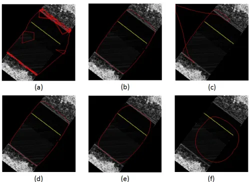
κ4 = 2in each test case. A proper analysis of the internal energy parameters requires that the movement of snake curve is to the left and right edges. Keeping this in mind, we empirically selected those values of external energy parameters which would enable the snake to reach the road edges. In each test case, we applied our road edge extraction algorithm to the road section. The final positions of the snake curve in the six test cases are shown in Figure2.

Fig. 2. Final position of the snake curve is represented in red over the slope raster surface in the (a) first, (b) second, (c) third, (d) fourth, (e) fifth, (f) sixth and (g) seventh test case of internal energy analysis, while the navigation points are represented in yellow.

In the first case, we started with the lowest possible values for the α, βandγ parameters. This caused the snake curve to be jagged at most of the points, as shown in Figure2(a). In the second case, the value ofαwas increased to 9along withβ= 0 andγ = 1 which caused the snake curve to move towards the road edges without any jaggedness, as shown in Figure 2(b). The α parameter is used to hold the snake curve together and control its elasticity. Its higher value increased the binding energy in the snake curve while its lower value caused the snake curve to move without any binding energy. Based on this analysis, we selected an optimal value of9for theα parameter when extracting the road edges.

In the third case, the value ofβwas increased to9along with an optimal value ofα and γ = 1. The effect on the snake curve was extreme binding at some of its points, as can be seen in Figure2(c). In the fourth case, we set the minimum value of theβ parameter to

but its higher value caused extreme bending in the snake curve. The extraction of the road edge does not require much bending in the snake curve so a low value of0.001was found to be optimal for the β parameter.

In the fifth case, we increased the value ofγparameter to3along with optimal values of α and β which enabled the snake curve to accurately converge to the road edges, as can be seen in Figure2(e). In the sixth case, the γ parameter value was further increased to9

along with optimal values for the other internal energy terms. These changes obstructed the movement of the snake curve towards the road edges, as shown in Figure 2(f). The γ parameter controls the step size of the snake curve in one iteration. The higher value led to the controlled step size of the snake curve in one iteration obstructing its growth, while a lower value led to the relatively less controlled step size of the snake curve in one iteration causing its free movement beyond the left edge as in the second and fourth cases. Thus, an optimal value ofγparameter was selected as3for extracting the road edges. This internal energy analysis helped us to understand that the lower values of β and γ parameters are required while a relatively higher value of theαparameter is required to force the snake curve to converge more precisely to the road edges. These findings enabled us to select the optimal values of the internal energy parameters in a more efficient and simplified way.

B. External Energy

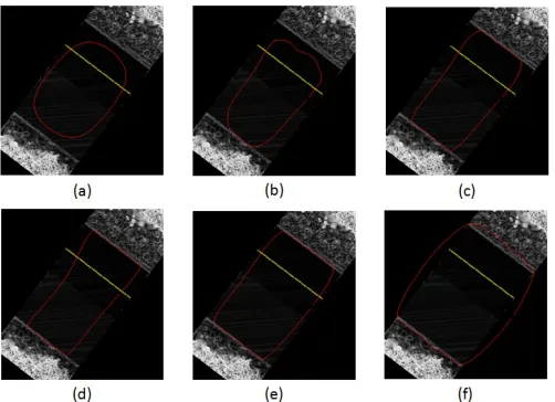
In this section we considered six test cases in which the per-formance of our algorithm was analysed with the use of various combinations of κ1, κ2, κ3 and κ4 external energy parameters, as shown in shown in Table III. The internal energy parameters were selected as α = 9, β = 0.001 and γ = 3. We applied our road edge extraction algorithm in each test case. The final positions of the snake curve in the six test cases are shown in Figure3. In the first

TABLE III

THE VALUES OFκ1, κ2, κ3ANDκ4WEIGHT PARAMETERS USED IN THE SIX TEST CASES OF EXTERNAL ENERGY ANALYSIS.

Test Case κ1 κ2 κ3 κ4

1 0 4 0 0

2 0 4 2 0

3 0 4 2 2

4 0 4 4 4

5 1 4 2 2

6 4 4 2 2

case of the external energy analysis, we initiated the process with a κ2 = 4 weight which provided only a slope based GVF energy. The applied energy caused the snake curve to move towards the road edges, however, it was not sufficiently strong to force the snake cuve to reach the edges, as shown in Figure 3(a). In the second case, we set κ3 = 2, the weight to reflectance based GVF energy, along with κ2 = 4. This caused the snake curve to move further towards the road edges compared with its position in the first case, as can be seen in Figure 3(b). In the third case, the κ4 = 2 weight was set for the pulse width based GVF energy along with κ2 = 4 and

κ3= 2. This caused the snake curve to converge to both the left and right edges, as shown in Figure3(c). In the fourth case, we provided equal weights to the slope, reflectance and pulse width based GVF energy terms with κ2= 4, κ3 = 4and κ4= 4, however, the snake curve was not able to efficiently converge to the road edges as can be seen in the third test case, shown in Figure 3(d). The reflectance values provided by the laser scanner in the XP-1 MLS system are not accurately normalised which leads to different values over the road surface. The hierarchical thresholding applied to the reflectance raster

Fig. 3. Final position of the snake curve is represented in red over the slope raster surface in the (a) first, (b) second, (c) third, (d) fourth, (e) fifth and (f) sixth case of external energy parameter analysis, while the navigation points are represented in yellow.

surface failed to remove the road marking cells near the left road edge which obstructed the snake curve preventing it from moving beyond them. Due to its imperfect normalisation, we decided to keep the lower weight for the reflectance based GVF energy than slope GVF energy. Similarly, we did not chose to set the highest weight to the pulse width based GVF energy because the orientation of the kerb edges relative to the vehicle is similar to that of the road surface. This together with their similar surface composition results in the pulse width having similar values which leads to lower priority for the pulse width attribute in urban regions. Based on this, we selected optimal values forκ2, κ3 and κ4 as 4, 2 and 2 respectively in the third case.

In the fifth case, the balloon energy was included in the external energy with κ1 = 1 along with an optimal values for other GVF energy terms. The balloon energy pushed the snake curve outwards causing it to converge to the road edges better than in the third case, as shown in Figure3(e). In the sixth case, we increased the value ofκ1 balloon energy weight to4along with an optimal values for other GVF energy terms. The snake curve fully converged to the road edges but also moved beyond the left and right edges as shown in Figure 3(f). Thus, we selected an optimal value for κ1 as 1. However, an increased weight to the balloon energy can be useful in cases of noisy data along the road section which provides an additional inflation energy to the snake curve to overcome the noise. This experimental analysis demonstrated the relative importance of GVF and balloon external energy terms in our algorithm and enabled us to efficiently estimate their optimal values. In the next section, we present a modified balloon external energy in our road edge extraction algorithm.

V. BALLOONENERGYMODIFICATION

Fig. 4. Final position of the snake curve is represented in red over the slope raster surface with (a)κ1= 1and (b)κ1 = 4parameter in10m national primary road section, while the navigation points are represented in yellow.

Fig. 5. (a) Initial and (b) final position of the snake curve is represented in red over the slope raster surface withκlef t₁ = 1andκright₁ = 4in a10m national primary road section, navigation points are represented in yellow while end points of major axis of the initial snake curve are represented as white dots.

with a lower point density along the right side of the road section than along its left side. It resulted in a large number of noisy cells along the right side of the road section in the slope raster surface generated from the LiDAR elevation attribute. This noise can be overcome by providing an increased weight to the balloon energy parameter with κ1= 4. It provides an additional inflation energy to the snake curve to move it towards the right road edge, as shown in Figure4(b). However, the increased balloon energy pushes the snake curve beyond the weak left edge points. This limitation can also be overcome with a modified balloon energy in our road edge extraction algorithm.

We modified the balloon energy by providing a low balloon energy weight to the snake points toward the left side of the road section while keeping a high weight to the snake points toward the right side of the road section. In this process, end points of major axis of the initial snake curve were first estimated as shown in Figure5(a). In each iteration of the algorithm, the snake points nearest to the end points were estimated and then the selected snake points were used to divide the snake curve points into the points toward left and right side of the road section. Finally, the balloon energy withκlef t1 = 1was provided to the snake points toward the left side while the balloon energy with κright1 = 4 was provided to the snake points toward the right side. During an iterative process, the snake curve moved towards the left and right edges of the road section and converged efficiently to them, as shown in Figure 5(b). The left-side balloon energy kept the snake from moving beyond the left edge while the right-side balloon energy provided an additional inflation energy to the snake curve to move towards the right edge. In this way, the use of balloon energy weight parameter was balanced relative to the non-uniform point density of the LiDAR data. In the next section, we present our approach for validating the road edges extracted from MLS data.

VI. ROADEDGEVALIDATIONAPPROACH

This section details an approach for validating the road edges extracted from MLS data. This approach is based on an automated estimation of the road edge’s orthogonal proximity from a reference road edge. The reference edge can be based on either manual digiti-sation or a ground truth data collected using field survey. As is shown in Figure 6(a), an automated estimation of the orthogonal distance Ain between the original positions of extracted and reference road edge points would be more complex. This is because the orthogonal

Fig. 6. Road edge validation approach: (a) Original and (b) rotated positions of extracted and reference road edges, where red represents the extracted road edges, blue represents the reference road edges, yellow represents the navigation points and green represents the navigation point selected in each iteration.

position of the reference edge point with respect to any selected extracted edge point is not known. In order to simplify the process of estimating orthogonal distance, the points are rotated towards the horizontal axis based on the navigation data, which provides the heading angle information of the road section with respect to true North.

VII. EXPERIMENTATION

We selected three complex sections of road to test our road edge extraction algorithm. These sections covered 245m of road which consisted of distinct sets of edges, roundabout and high degree of curvature. The first50m section of minor road consisted of a grass-soil edge along its left side and a kerb edge along its right side as shown in Figure 7(a). The second 105m section of primary route

Fig. 7. Digital image of the (a) first road section consisting of a grass-soil edge along its left side and a kerb edge along its right side in County Nottinghamshire, UK (Geographic location: 53◦01000.0800N 0◦54006.300W) (Image Courtesy: StreetMapper), (b) second road section consisting of kerb edges along both sides of a roundabout in County Gloucestershire, UK (Geo-graphic location: 51◦43002.200N 1◦57035.300W) (Image Courtesy: Streetview, Google) and (c) third road section consisting of grass-soil edges along both sides with a high degree of curvature in County Westmeath, Ireland (Geo-graphic location: 53◦₃₃0_26.300_{N 7}◦₁₃0_29.700_{W) (Image Courtesy: Ubipix).}

network consisted of kerb edges along both sides of a roundabout as shown in Figure7(b) while the third90m section of national primary road consisted of grass-soil edges along both sides with a high degree of curvature, as shown in Figure 7(c). The lengths of these road sections were selected such that the distinct edges, roundabout and high degree of curvature features could be included in our algorithm tests. The processed datasets for the first, second and third road sections were acquired using StreetMapper [31], RouteMapper [32] and XP-1 MLS systems respectively. These datasets, from multiple MLS systems, were selected to validate the robustness of our algorithm. To process 50m, 105m and90m road sections, we used n= 6,13and 11 sets of30m×10m×5m sections of LiDAR data respectively. While n = 6,13and 11sets of10m sections of navigation data, respectively were used.

The parameters used in our algorithm are shown in TableIV. In

TABLE IV

THE PARAMETERS USED IN THE AUTOMATED ROAD EDGE EXTRACTION ALGORITHM.

Parameter Value Parameter Value Parameter Value

c 0.06 m2 _T

int 55 κ2 4

Mslope 5 Tpw 10 κ3 2

Mref 5 T1 250 κ4 2

Mint 5 T2 5 ω 20◦

Mpw 5 α 9 δλ 0.03

Tslope 45 β 0.001 µ 0.2

Tref 95 γ 3

the first road section, the acquired data contained intensity values which enabled us to use the mask size, Mint and threshold Tint

parameters in our algorithm. The data did not included a pulse width attribute, thus, our algorithm was applied based on elevation and intensity attributes only. In the second road section, the algorithm was applied based on only elevation and pulse width attributes while in the third road section, we used elevation, reflectance and pulse width attributes. The value of φ was calculated from the average heading angle,θ of the survey vehicle along each road section. The number of GVF iterations was600, while the number of iterations required to move the snake curve was 40.

In the first road section, the data was acquired using a single laser scanner with a double-pass approach in which the vehicle was driven back and forth on the road section. This led to uniform and dense point cloud data along the first road section in comparison with the second and third road sections, where the data was acquired using a single laser scanner and only a single-pass approach. Moreover, we did not utilised the reflectance attribute in the second road section due to which the snake curve was not able to converge fully to the road edges in most of the cases. This caused us to apply a modified balloon energy withκlef t1 = 1 and κ

right

1 = 2in the second road section. In the first road section, the point density was uniform and dense while in the third road section, we utilised all the LiDAR attributes, allowing us to define the balloon energy withκlef t₁ = 1

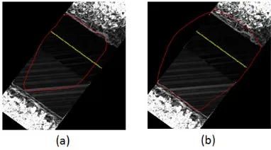
and κright1 = 1. We applied our automated road edge extraction to each road section with the optimally selected parameters. We also manually digitised the left and right edges from the 3D LiDAR data in each road section. The automated extracted 3D edges are represented in red while the manually digitised 3D edges are represented in blue in the first, second and third road sections in Figures8, 9 and 10

respectively. In the next section, we validate the experimental results

Fig. 8. The automatically extracted 3D edges are represented in red and the manually digitised 3D edges are represented in blue in the first50m road section. The inset pictures of (a) left and (b) right edges show some of the points in detail.

Fig. 9. The automatically extracted 3D edges are represented in red and the manually digitised 3D edges are represented in blue in the second105m road section. The inset pictures (a) and (b) of left and right edges show some of the points in detail.

using our road edge validation approach and discuss them.

VIII. RESULTS AND DISCUSSION

Fig. 10. The automatically extracted 3D edges are represented in red and the manually digitised 3D edges are represented in blue in the third 90m road section. The inset pictures (a) and (b) of left and right edges show some of the points in detail.

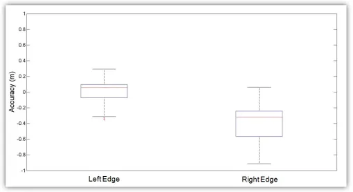
Box plots for the accuracy values of these extracted left and right edges in the first, second and third road sections are shown in Figures

11,12 and 13respectively. We also carried out statistical analyses

Fig. 11. Box plot for the accuracy values of the automatically extracted left and right edges in the first50m road section.

Fig. 12. Box plot for the accuracy values of the automatically extracted left and right edges in the second105m road section.

of the accuracy values for these extracted left and right edges in the first, second and third road sections as shown in Tables V and VI

respectively.

Our automated algorithm successfully extracted the left and right edges in all three road sections. In the first road section, accuracy values were found to be better than in the second and third road sections. The minimum-maximum and lower-upper adjacent range values were found to be lowest in the first section, while its left and

Fig. 13. Box plot for the accuracy values of the automatically extracted left and right edges in the third90m road section.

Left Edge First Section Second

Sec-tion

Third Section

minimum (m) -0.169 -0.351 -0.786

maximum (m) 0.170 0.292 0.868

lower adjacent (m) -0.134 -0.311 -0.248 upper adjacent (m) 0.086 0.292 0.622 25th percentile (m) -0.060 -0.073 -0.095 75th percentile (m) 0.11 0.096 0.259

mean (m) -0.020 0.008 0.071

median (m) -0.016 0.057 -0.014

outliers (%) 5.08 1.57 1.82

inside±0.01(%) 20.34 3.94 1.82

inside±0.1(%) 89.83 55.91 36.36

inside±0.2(%) 100 86.61 64.55

inside±0.3(%) 100 96.85 83.64

outside±0.3(%) 0 3.15 16.36

horizontal RMSE(m) 0.047 0.128 0.23

vertical RMSE(m) 0.048 0.043 0.097

TABLE V

STATISTICAL ANALYSIS OF THE ACCURACY VALUES OF THE AUTOMATICALLY EXTRACTED LEFT EDGES IN THE FIRST,SECOND AND

THIRD ROAD SECTIONS.

right edge accuracy values were within a±0.2m and±0.3m tolerance respecitvely. In the second road section,3.15%left edge and54.33%

right edge accuracy values were more than±0.3m tolerance, while in the third road section, 16.36% left edge and53.64%right edge accuracy values were found to be outside the±0.3m tolerance. The higher accuracy level in the first road section was attained due to the uniform and dense point cloud along it, which led to the generation of smooth raster surfaces. The use of such data enabled the snake curve to precisely converge to the road edges.

In the first road section, the left edge displayed slightly better results than the right edge. The minimum-maximum and lower-upper adjacent range values were higher for the right edge however, the percentages of accuracy inside ±0.01m, ±0.1m and ±0.2m were higher for the left edge. The accuracy level in the first section can be further improved with the use of a reflectance attribute which is a representation of the normalised intensity values. The intensity values are required to be normalised with respect to illuminated surface characteristics, distance from the laser scanner to the illuminated surface and incidence angle of the laser pulse [33]. This will allow us to assign a height weight to the reflectance GVF energy in the algorithm. The use of a pulse width attribute will also improve the accuracy values in the first road section.

Right Edge First Section Second

Sec-tion

Third Section

minimum (m) -0.280 -0.915 -0.556

maximum (m) -0.070 0.061 0.993

lower adjacent(m) -0.206 -0.915 -0.033 upper adjacent(m) -0.070 0.061 0.634 25th percentile(m) -0.146 -0.564 0.216 75th percentile (m) -0.104 -0.242 0.384

mean (m) -0.133 -0.384 0.303

median (m) -0.126 -0.320 0.309

outliers (%) 5.08 0 10

inside±0.01(%) 0 0.79 0

inside±0.1(%) 20.34 10.24 8.18

inside±0.2(%) 91.53 21.26 16.36

inside±0.3(%) 100 45.67 46.36

outside±0.3(%) 0 54.33 53.64

horizontal RMSE(m) 0.135 0.423 0.305

vertical RMSE(m) 0.028 0.155 0.24

TABLE VI

STATISTICAL ANALYSIS OF THE ACCURACY VALUES OF THE AUTOMATICALLY EXTRACTED RIGHT EDGES IN THE FIRST,SECOND AND

THIRD ROAD SECTIONS.

left edge, while in the third section, these range values were similar for both the left and right edges. In both these sections, the highest percentages of accuracy inside ±0.01m, ±0.1m and ±0.2m were the left edges. This lower accuracy for the right edge was due to lower point density along the right side. The use of a modified balloon energy in the second road section provided an additional inflation energy to the snake curve causing it to move towards the right edge however, it was not helpful in precisely converging the snake curve to the right edge. In the second section, the snake curves were found to be extended along the road-lanes entering into the roundabout. The non-road edge points in the extended snake curves can be automatically removed with the batch processing of entering road-lanes. In the third road section, the reflectance values were not accurately normalised which led to the generation of raster surfaces with road marking cells near the edges. It created an obstruction for the snake curve to move beyond them. The use of a properly normalised reflectance attribute along with a uniform and dense point cloud will provide an improved extraction of road edges in both the sections.

Yang et al. [21] and Wang et al. [24] validated the kerb edges extracted from MLS data by detailing an average completeness values of95.13% and95.41% respectively while average correctness values of 97.04% and 99.35% respectively. Guan et al. [23] reported an average horizontal and vertical Root Mean Square Error (RMSE) values of 0.081m and 0.021m respectively for the kerb edges extracted from MLS data. In comparison, our validation approach provided a more qualitative evaluation of extracted kerb edges based on estimating their orthogonal proximity from the manually digitised edges. Our automated algorithm extracted the kerb edges along right side of first road section and along both sides of second road section with an average horizontal and vertical RMSE values of0.229m and

0.075m respectively. This accuracy can be further improved with the use of dense point cloud data along both sides of road section and proper utilisation of all the LiDAR attributes in our algorithm.

We analysed the computational performance of our algorithm by estimating the total time taken by the snake curve to move from its initial position to the final position in each tested road section. In the first, second and third road sections, the snake curve took an approximate624,1357and864seconds respectively to converge to the road edges. This analysis was performed on a computer with Intel Core i7-4610M processor @3GHz,8GB RAM and a64-bit operating system.

IX. CONCLUSION

Our algorithm is based on the novel integration of GVF and balloon snake models to extract road edges from mobile laser scanning data. The algorithm was tested on datasets which were acquired using multiple MLS systems along complex road sections. The successful extraction of road edges from the sections consisting of distinct sets of edges, a roundabout and a high degree of curvature validates our algorithm. We presented a detailed analysis of the internal and external energy parameters involved in our algorithm. The use of these optimal values enabled automation of the process of extracting road edges for all the tested road sections. We modified the balloon external energy and presented its utility for extracting road edges from the datasets with low and non-uniform point densities. Our novel road edge validation approach negated various limitations associated with traditional approaches which are based on computing quality measure values with respect to buffer zones created around reference data. The presented approach enables us to efficiently validate the extracted edges in the tested road sections by directly estimating their orthogonal proximity from the reference edges.

The performance of our algorithm improved significantly with dense and uniform point cloud along the road sections. It could be further improved with the use of a reflectance attribute with proper normalised values. This will help distinguish the road surface from the grass-soil and the kerb edges more accurately. Further research is required to investigate the applicability of the geometric active contour models for extracting road edges. This could be advantageous as it will remove the requirement for weighting various input parameters. The urban road sections are often accompanied with stationary vehicles or pedestrians during the data acquisition process which can lead to missing points in the LiDAR data section. The missing points introduce noisy cells along the raster surface generated from the LiDAR data. This noise can be removed with an optimal use of hierarchical thresholding and modified balloon energy approaches which are required to be further analysed. We intend to develop an error correction approach which, when incorporated in our algorithm will remove false road edges caused by false positives or occlusions. Large scale implementation of our algorithm will be enabled through the ongoing construction of a geospatial data management system to handle 100s of kms of LiDAR data.

ACKNOWLEDGEMENTS

Research presented in this paper was initially funded by the Irish Research Council Enterprise Partnership scheme and Strategic Research Cluster grants (07/SRC/I1168 & 13/IF/I2782) of Science Foundation Ireland under the National Development Plan. The re-search is continued at Universiti Teknologi Malaysia. The authors gratefully acknowledge this support. The authors also acknowledge the 3D Laser Mapping company for providing the Streetmapper mobile laser scanning data.

REFERENCES

[1] WHO, “Global status report on road safety,” Available:

http://www.who.int/violence injury prevention/road safety status,

2013.

[2] G. Gatti, C. Polidori, I. Galvez, K. Mallschutzke, R. Jorna, M. Leur, M. Dietze, D. Ebersbach, C. Lippold, B. Schlag, G. Weller, A. Wyczynski, F. Iman, and C. Aydin, “Safety handbook for secondary roads,” Available:

http://ec.europa.eu/transport/roadsafety library, 2007.

[3] UNECE, “Transport review: road safety,” Available:

http://www.unece.org, 2008.

[5] T. McCarthy and C. P. McElhinney, “European Road Safety Inspection (EuRSI) research project,”Proc. European Transport

Conference, Glasgow, 11-13 October, 2010.

[6] P. Kumar, C. P. McElhinney, P. Lewis, and T. McCarthy, “An automated algorithm for extracting road edges from terrestrial mobile LiDAR data,” ISPRS Journal of Photogrammetry and

Remote Sensing, vol. 85, pp. 44–55, 2013.

[7] M. Kass, A. Witkin, and D. Terzopoulos, “Snakes: Active contour models,” International Journal of Computer Vision, vol. 1, no. 4, pp. 321–331, 1988.

[8] P. Kumar, “Road features extraction using terrestrial mobile laser scanning system,”Ph.D. Dissertation, National University

of Ireland Maynooth, p. 300, 2012.

[9] V. Caselles, F. Catt, T. Coll, and F. Dibos, “A geometric model for active contours in image processing,” Numerische

Mathematik, vol. 66, pp. 1–31, 1993.

[10] R. Malladi, J. A. Sethian, and B. C. Vemuri, “Shape modeling with front propagation: a level set approach,”IEEE Transactions

on Pattern Analysis and Machine Intelligence, vol. 17, no. 2,

pp. 158–175, 1995.

[11] G. Vosselman and Z. Liang, “Detection of curbstones in airborne laser scanning data,”International Archives of Photogrammetry,

Remote Sensing and Spatial Information Sciences, vol. 38, no.

Part 3/W8, pp. 111–116, 2009.

[12] C. Heipke, H. Mayer, C. Wiedemann, and O. Jamet, “Evaluation of automatic road extraction,”International Archives of

Pho-togrammetry, Remote Sensing and Spatial Information Sciences,

vol. 32, no. Part 2/3W3, pp. 151–160, 1997.

[13] S. J. O. Elberink and G. Vosselman, “Quality analysis of 3D road reconstruction,” International Archives of the

Pho-togrammetry, Remote Sensing and Spatial Information Sciences,

vol. 36, no. Part 3/W52, pp. 1–6, 2007.

[14] S. O. Elberink and G. Vosselman, “3D information extraction from laser point clouds covering complex road junctions,”The

Photogrammetric Record, vol. 24, no. 125, pp. 23–36, 2009.

[15] A. Jaakkola, J. Hyypp¨a, H. Hyypp¨a, and A. Kukko, “Retrieval algorithms for road surface modelling using laser based mobile mapping,”Sensors, vol. 8, no. 9, pp. 5238–5249, sep 2008. [16] J. Goepfert and F. Rottensteiner, “Adaption of roads to ALS

data by means of network snakes,” International Archives of Photogrammetry, Remote Sensing and Spatial Information

Sci-ences, vol. 38, no. 3/W8, pp. 24–29, 2009.

[17] A. Boyko and T. Funkhouser, “Extracting roads from dense point clouds in large scale urban environment,”ISPRS Journal

of Photogrammetry and Remote Sensing, vol. 66, no. 6, pp. S2–

S12, 2011.

[18] S. Ibrahim and D. Lichti, “Curb-based street floor extrac-tion from mobile terrestrial LiDAR point cloud,”International Archives of Photogrammetry, Remote Sensing and Spatial

In-formation Sciences, vol. 39, no. Part B5, pp. 193–198, 2012.

[19] L. Zhou and G. Vosselman, “Mapping curbstones in airborne and mobile laser scanning data,”International Journal of

Ap-plied Earth Observation and Geoinformation, vol. 18, pp. 293–

304, 2012.

[20] A. Serna and B. Marcotegui, “Urban accessibility diagnosis from mobile laser scannning data,” ISPRS Journal of

Pho-togrammetry and Remote Sensing, vol. 84, pp. 23–32, 2013.

[21] B. Yang, L. Fang, and J. Li, “Semi-automated extraction and delineation of 3D roads of street scene from mobile laser scanning point clouds,”ISPRS Journal of Photogrammetry and

Remote Sensing, vol. 79, pp. 80–93, 2013.

[22] H. Guan, J. Li, Y. Yu, C. Wang, M. Chapman, and B. Yang, “Using mobile laser scanning data for automated extraction of

road markings,”ISPRS Journal of Photogrammetry and Remote

Sensing, vol. 87, pp. 93–107, 2014.

[23] H. Guan, J. Li, Y. Yu, M. Chapman, and C. Wang, “Auto-mated road information extraction from mobile laser scanning data,”IEEE Transactions on Intelligent Transportation Systems, vol. 16, no. 1, pp. 194–205, 2015.

[24] H. Wang, H. Luo, C. Wen, J. Cheng, P. Li, Y. Chen, C. Wang, and J. Li, “Road boundaries detection based on local normal saliency from mobile laser scanning data,”IEEE Geoscience and

remote sensing letters, vol. 12, no. 10, pp. 2085–2089, 2015.

[25] P. Kumar, P. Lewis, and C. P. McElhinney, “Parametric analysis for automated extraction of road edges from mobile laser scanning data,” International Annals of the Photogrammetry,

Remote Sensing and Spatial Information Sciences, vol. II-2/W2,

pp. 215–221, 2015.

[26] C. Crawford, “Minimizing noise from LiDAR for contouring and slope analysis,” Available:

http://blogs.esri.com/esri/arcgis/2009/09/02, 2009.

[27] ESRI, “Terrain pyramids,” Available:

http://webhelp.esri.com/ArcGISdesktop/9.3, 2010.

[28] C. Xu and J. L. Prince, “Gradient vector flow: a new external force for snakes,”Proc. Computer Vision Pattern Recognition,

San Juan, US, pp. 66–71, 1997.

[29] M. Sonka, V. Hlavac, and R. Boyle,Image processing, analysis

and machine vision. Second edition, Thomson Engineering,

New York, 2008.

[30] J. Canny, “A computational approach to edge detection,”IEEE

Transactions on Pattern Analysis and Machine Intelligence,

vol. 8, no. 6, pp. 679–698, 1986.

[31] StreetMapper, “3D laser mapping,” Available:

http://www.3dlasermapping.com/streetmapper, 2015.

[32] RouteMapper, “IBI Group,” Available:

http://www.routemapper.net, 2015.