Learning Structured Models for Phone Recognition

Learning Structured Models for Phone Recognition

Slav Petrov Adam Pauls Dan Klein

Computer Science Department, EECS Divison University of California at Berkeley

Berkeley, CA, 94720, USA

{petrov,adpauls,klein}@cs.berkeley.edu

Abstract

We present a maximally streamlined approach to learning HMM-based acoustic models for automatic speech recognition. In our approach, an initial mono-phone HMM is iteratively refined using a split-merge EM procedure which makes no assumptions about subphone structure or context-dependent structure, and which uses only a single Gaussian per HMM state. Despite the much simplified training process, our acoustic model achieves state-of-the-art results on phone classification (where it outperforms almost all other methods) and competitive performance on phone recognition (where it outperforms standard CD triphone / subphone / GMM approaches). We also present an analysis of what is and is not learned by our system.

1 Introduction

Continuous density hidden Markov models (HMMs) underlie most automatic speech recognition (ASR) systems in some form. While the basic algorithms for HMM learning and inference are quite general, acoustic models of speech standardly employ rich speech-specific structures to improve performance. For example, it is well known that a monophone HMM with one state per phone is too coarse an approximation to the true articulatory and acoustic process. The HMM state space is therefore refined in several ways. To model phone-internal dynam-ics, phones are split intobeginning,middle, andend subphones (Jelinek, 1976). To model cross-phone coarticulation, the states of the HMM are refined by splitting the phones into context-dependent tri-phones. These states are then re-clustered (Odell, 1995) and the parameters of their observation dis-tributions are tied back together (Young and Wood-land, 1994). Finally, to model complex emission

densities, states emit mixtures of multivariate Gaus-sians. This standard structure is shown schemati-cally in Figure 1. While this rich structure is pho-netically well-motivated and empirically success-ful, so much structural bias may be unnecessary, or even harmful. For example in the domain of syn-tactic parsing with probabilistic context-free gram-mars (PCFGs), a surprising recent result is that au-tomatically induced grammar refinements can out-perform sophisticated methods which exploit sub-stantial manually articulated structure (Petrov et al., 2006).

In this paper, we consider a much more automatic, data-driven approach to learning HMM structure for acoustic modeling, analagous to the approach taken by Petrov et al. (2006) for learning PCFGs. We start with a minimal monophone HMM in which there is a single state for each (context-independent) phone. Moreover, the emission model for each state is a sin-gle multivariate Gaussian (over the standard MFCC acoustic features). We then iteratively refine this minimal HMM through state splitting, adding com-plexity as needed. States in the refined HMMs are always substates of the original HMM and are there-fore each identified with a unique base phone. States are split, estimated, and (perhaps) merged, based on a likelihood criterion. Our model never allows ex-plicit Gaussian mixtures, though substates may de-velop similar distributions and thereby emulate such mixtures.

In principle, discarding the traditional structure can either help or hurt the model. Incorrect prior splits can needlessly fragment training data and in-correct prior tying can limit the model’s expressiv-ity. On the other hand, correct assumptions can increase the efficiency of the learner. Empirically,

Start begin mid end begin mid end End

d₇= c(#-d-ae)

begin mid end begin mid end ae₃= c(d-ae-d) d₁₃= c(ae-d-#)

Start

a d

End

a d a d

d ae d

b c b c b c

Figure 1: Comparison of the standard model to our model (here shown withk = 4subphones per phone) for the word dad. The dependence of subphones across phones in our model is not shown, while the context clustering in the standard model is shown only schematically.

we show that our automatic approach outperforms classic systems on the task of phone recognition on the TIMIT data set. In particular, it outperforms standard state-tied triphone models like Young and Woodland (1994), achieving a phone error rate of 26.4% versus 27.7%. In addition, our approach gives state-of-the-art performance on the task of phone classification on the TIMIT data set, suggest-ing that our learned structure is particularly effec-tive at modeling phone-internal structure. Indeed, our error rate of 21.4% is outperformed only by the recent structured margin approach of Sha and Saul (2006). It remains to be seen whether these posi-tive results on acoustic modeling will facilitate better word recognition rates in a large vocabulary speech recognition system.

We also consider the structures learned by the model. Subphone structure is learned, similar to, but richer than, standard begin-middle-end struc-tures. Cross-phone coarticulation is also learned, with classic phonological classes often emerging naturally.

Many aspects of this work are intended to sim-plify rather than further articulate the acoustic pro-cess. It should therefore be clear that the basic tech-niques of splitting, merging, and learning using EM are not in themselves new for ASR. Nor is the basic latent induction method new (Matsuzaki et al., 2005; Petrov et al., 2006). What is novel in this paper is (1) the construction of an automatic system for acous-tic modeling, with substantially streamlined struc-ture, (2) the investigation of variational inference for such a task, (3) the analysis of the kinds of struc-tures learned by such a system, and (4) the empirical

demonstration that such a system is not only com-petitive with the traditional approach, but can indeed outperform even very recent work on some prelimi-nary measures.

2 Learning

In the following, we propose a greatly simplified model that does not impose any manually specified structural constraints. Instead of specifying struc-turea priori, we use the Expectation-Maximization (EM) algorithm for HMMs (Baum-Welch) to auto-matically induce the structure in a way that maxi-mizes data likelihood.

In general, our training data consists of sets of acoustic observation sequences and phone level transcriptionsrwhich specify a sequence of phones from a set of phones Y, but does not label each time frame with a phone. We refer to an observa-tion sequence asx = x1, . . . , xT wherexi ∈ R39

are standard MFCC features (Davis and Mermel-stein, 1980). We wish to induce an HMM over a set of states S for which we also have a function π : S → Y that maps every state in S to a phone inY. Note that in the usual formulation of the EM algorithm for HMMs, one is interested in learning HMM parametersθthat maximize the likelihood of the observations P(x|θ); in contrast, we aim to max-imize the joint probability of our observations and phone transcriptions P(x,r|θ) or observations and phone sequences P(x,y|θ)(see below). We now de-scribe this relatively straightforward modification of the EM algorithm.

2.1 The Hand-Aligned Case

For clarity of exposition we first consider a simpli-fied scenario in which we are given hand-aligned phone labelsy = y1, . . . , yT for each timet, as is

the case for the TIMIT dataset. Our procedure does not require such extensive annotation of the training data and in fact gives better performance when the exact transition point between phones are not pre-specified but learned.

next previous th dh p t b g dx w r l s z sh f cl vcl m n ng l r er 0 (a) next previous th dh p t b g dx w r l s z sh f cl vcl m n ng l r er 0 1 (b) next previous th dh p t b g dx w r l s z sh f cl vcl m n ng l r er 0 3 2 1 (c) next previous th dh p t b g dx w r l s z sh f cl vcl m n ng l r er 1 6 0 3 4 7 2 5 (d) Figure 2: Iterative refinement of the /ih/ phone with1,2,4,8substates.

ending in statesat timet:

αt(s) =P(x1, . . . , xt, y1, . . . yt, st=s|λ),

and the backward probability is the probability of observing the sequencext+1, . . . , xT with

transcrip-tion yt+1, . . . , yT, given that we start in states at

timet:

βt(s) =P(xt+1, . . . , xT, yt+1, . . . , yT|st=s, λ),

where λ are the model parameters. As usual, we parameterize our HMMs with ass0, the probability

of transitioning from state s to s0, and bs(x) ∼ N(µs,Σs), the probability emitting the observation

xwhen in states.

These probabilities can be computed using the standard forward and backward recursions (Rabiner, 1989), except that at each time t, we only con-sider states st for which π(st) = yt, because we

have hand-aligned labels for the observations. These quantities also allow us to compute the posterior counts necessary for the E-step of the EM algorithm.

2.2 Splitting

One way of inducing arbitrary structural annota-tions would be to split each HMM state in into msubstates, and re-estimate the parameters for the split HMM using EM. This approach has two ma-jor drawbacks: for largermit is likely to converge to poor local optima, and it allocates substates uni-formly across all states, regardless of how much an-notation is required for good performance.

To avoid these problems, we apply a hierarchical parameter estimation strategy similar in spirit to the work of Sankar (1998) and Ueda et al. (2000), but here applied to HMMs rather than to GMMs. Be-ginning with the baseline model, where each state corresponds to one phone, we repeatedly split and re-train the HMM. This strategy ensures that each split HMM is initialized “close” to some reasonable maximum.

Concretely, each state s in the HMM is split in two new statess1, s2 withπ(s1) = π(s2) = π(s).

We initialize EM with the parameters of the previ-ous HMM, splitting every previprevi-ous state s in two and adding a small amount of randomness ≤ 1% to its transition and emission probabilities to break symmetry:

as1s0 ∝ass0+,

bs1(o) ∼ N(µs+,Σs),

and similarly fors2. The incoming transitions are

split evenly.

We then apply the EM algorithm described above to re-estimate these parameters before performing subsequent split operations.

2.3 Merging

sub-states only where needed, rather than splitting them all.

We realize this goal by merging back those splits s → s1s2 for which, if the split were reversed, the

loss in data likelihood would be smallest. We ap-proximate the loss in data likelihood for a merge s1s2 →swith the following likelihood ratio (Petrov

et al., 2006):

∆(s1s2 →s) = Y

sequences Y

t

Pt(x,y) P(x,y).

Here P(x,y) is the joint likelihood of an emission sequence x and associated state sequencey. This quantity can be recovered from the forward and backward probabilities using

P(x,y) = X

s:π(s)=yt

αt(s)·βt(s).

Pt(x,y)is an approximation to the same joint like-lihood where states s1 ands2 are merged. We

ap-proximate the true loss by only considering merging statess1 ands2 at timet, a value which can be

ef-ficiently computed from the forward and backward probabilities. The forward score for the merged state sat timetis just the sum of the two split scores:

ˆ

αt(s) =αt(s1) +αt(s2),

while the backward score is a weighted sum of the split scores:

ˆ

βt(s) =p1βt(s1) +p2βt(s2),

wherep1 andp2are the relative (posterior)

frequen-cies of the statess1 ands2.

Thus, the likelihood after merging s1 and s2 at

timetcan be computed from these merged forward and backward scores as:

Pt(x,y) = ˆαt(s)·βˆt(s) + X

s0

αt(s0)·βt(s0)

where the second sum is over the other substates of xt, i.e. {s0 : π(s0) = xt, s0 ∈ {/ s1, s2}}. This

expression is an approximation because it neglects interactions between instances of the same states at multiple places in the same sequence. In particular,

since phones frequently occur with multiple consec-utive repetitions, this criterion may vastly overesti-mate the actual likelihood loss. As such, we also im-plemented the exact criterion, that is, for each split, we formed a new HMM withs1 ands2merged and

calculated the total data likelihood. This method is much more computationally expensive, requiring a full forward-backward pass through the data for each potential merge, and was not found to produce noticeably better performance. Therefore, all exper-iments use the approximate criterion.

2.4 The Automatically-Aligned Case

It is straightforward to generalize the hand-aligned case to the case where the phone transcription is known, but no frame level labeling is available. The main difference is that the phone boundaries are not known in advance, which means that there is now additional uncertainty over the phone states. The forward and backward recursions must thus be ex-panded to consider all state sequences that yield the given phone transcription. We can accomplish this with standard Baum-Welch training.

3 Inference

An HMM over refined subphone statess ∈ S nat-urally gives posterior distributions P(s|x) over se-quences of states s. We would ideally like to ex-tract the transcriptionrof underlying phones which is most probable according to this posterior1. The transcription is two stages removed from s. First, it collapses the distinctions between statesswhich correspond to the same phoney = π(s). Second, it collapses the distinctions between where phone transitions exactly occur. Viterbi state sequences can easily be extracted using the basic Viterbi algorithm. On the other hand, finding the best phone sequence or transcription is intractable.

As a compromise, we extract the phone sequence (not transcription) which has highest probability in a variational approximation to the true distribution (Jordan et al., 1999). Let the true posterior distri-bution over phone sequences be P(y|x). We form an approximation Q(y) ≈ P(y|x), where Q is an approximation specific to the sequencexand

factor-1

izes as:

Q(y) =Y

t

q(t, xt, yt+1).

We would like to fit the valuesq, one for each time step and state-state pair, so as to make Q as close to P as possible:

min

q KL(P(y|x)||Q(y)).

The solution can be found analytically using La-grange multipliers:

q(t, y, y0) = P(Yt=y, Yt+1=y

0_|x)

P(Yt=y|x)

.

where we have made the position-specific random variablesYtexplicit for clarity. This approximation

depends only on our ability to calculate posteriors over phones or phone-phone pairs at individual po-sitionst, which is easy to obtain from the state pos-teriors, for example:

P(Yt=y,Yt+1 =y0|x) = X

s:π(s)=y X

s0_:π(s0_)=y0

αt(s)ass0b_s0(x_t)β_t+1(s0)

P(x)

Finding the Viterbiphonesequence in the approxi-mate distribution Q, can be done with the Forward-Backward algorithm over the lattice ofqvalues.

4 Experiments

We tested our model on the TIMIT database, using the standard setups for phone recognition and phone classification. We partitioned the TIMIT data into training, development, and (core) test sets according to standard practice (Lee and Hon, 1989; Gunawar-dana et al., 2005; Sha and Saul, 2006). In particu-lar, we excluded allsasentences and mapped the 61 phonetic labels in TIMIT down to 48 classes before training our HMMs. At evaluation, these 48 classes were further mapped down to 39 classes, again in the standard way.

MFCC coefficients were extracted from the TIMIT source as in Sha and Saul (2006), includ-ing delta and delta-delta components. For all experi-ments, our system and all baselines we implemented usedfull covariancewhen parameterizing emission

0.24 0.26 0.28 0.3 0.32 0.34 0.36 0.38 0.4 0.42

0 200 400 600 800 1000 1200 1400 1600 1800 2000

Phone Recognition Error

Number of States split only split and merge split and merge, automatic alignment

Figure 3: Phone recognition error for models of increasing size

models.2 _{All Gaussians were endowed with weak}

inverse Wishart priors with zero mean and identity covariance.3

4.1 Phone Recognition

In the task of phone recognition, we fit an HMM whose output, with subsequent states collapsed, cor-responds to the training transcriptions. In the TIMIT data set, each frame is manually phone-annotated, so the only uncertainty in the basic setup is the identity of the (sub)states at each frame.

We therefore began with a single state for each phone, in a fully connected HMM (except for spe-cial treatment of dedicated start and end states). We incrementally trained our model as described in Sec-tion 2, with up to 6 split-merge rounds. We found that reversing 25% of the splits yielded good overall performance while maintaining compactness of the model.

We decoded using the variational decoder de-scribed in Section 3. The output was then scored against the reference phone transcription using the standard string edit distance.

During both training and decoding, we used “flat-tened” emission probabilities by exponentiating to some0 < γ < 1. We found the best setting forγ to be 0.2, as determined by tuning on the develop-ment set. This flattening compensates for the

non-2

Most of our findings also hold for diagonal covariance Gaussians, albeit the final error rates are 2-3% higher.

3

Method Error Rate State-Tied Triphone HMM

27.7%1 (Young and Woodland, 1994)

Gender Dependent Triphone HMM

27.1%1 (Lamel and Gauvain, 1993)

This Paper 26.4%

Bayesian Triphone HMM

25.6% (Ming and Smith, 1998)

Heterogeneous classifiers

24.4% (Halberstadt and Glass, 1998)

Table 1: Phone recognition error rates on the TIMIT core test from Glass (2003).

1_{These results are on a slightly easier test set.}

independence of the frames, partially due to over-lapping source samples and partially due to other unmodeled correlations.

Figure 3 shows the recognition error as the model grows in size. In addition to the basic setup de-scribed so far (split and merge), we also show a model in which merging was not performed (split only). As can be seen, the merging phase not only decreases the number of HMM states at each round, but also improves phone recognition error at each round.

We also compared our hierarchical split only model with a model where we directly split all states into2ksubstates, so that these models had the same number of states as a a hierarchical model after k split and merge cycles. While for smallk, the dif-ference was negligible, we found that the error in-creased by 1% absolute fork = 5. This trend is to be expected, as the possible interactions between the substates grows with the number of substates.

Also shown in Figure 3, and perhaps unsurprising, is that the error rate can be further reduced by allow-ing the phone boundaries to drift from the manual alignments provided in the TIMIT training data. The split and merge, automatic alignmentline shows the result of allowing the EM fitting phase to reposition each phone boundary, giving absolute improvements of up to 0.6%.

We investigated how much improvement in accu-racy one can gain by computing the variational ap-proximation introduced in Section 3 versus extract-ing the Viterbi state sequence and projectextract-ing that se-quence to its phone transcription. The gap varies,

Method Error Rate

GMM Baseline (Sha and Saul, 2006) 26.0% HMM Baseline (Gunawardana et al., 2005) 25.1% SVM (Clarkson and Moreno, 1999) 22.4% Hidden CRF (Gunawardana et al., 2005) 21.7%

This Paper 21.4%

Large Margin GMM (Sha and Saul, 2006) 21.1% Table 2: Phone classification error rates on the TIMIT core test.

but on a model with roughly 1000 states (5 split-merge rounds), the variational decoder decreases er-ror from 26.5% to 25.6%. The gain in accuracy comes at a cost in time: we must run a (possibly pruned) Forward-Backward pass over the full state spaceS, then another over the smaller phone space Y. In our experiments, the cost of variational decod-ing was a factor of about 3, which may or may not justify a relative error reduction of around 4%.

The performance of our best model (split and merge, automatic alignment, and variational decod-ing) on the test set is 26.4%. A comparison of our performance with other methods in the literature is shown in Table 1. Despite our structural simplic-ity, we outperform state-tied triphone systems like Young and Woodland (1994), a standard baseline for this task, by nearly 2% absolute. However, we fall short of the best current systems.

4.2 Phone Classification

Phone classification is the fairly constrained task of classifying in isolation a sequence of frames which is known to span exactly one phone. In order to quantify how much of our gains over the triphone baseline stem from modeling context-dependencies and how much from modeling the inner structure of the phones, we fit separate HMM models for each phone, using the same split and merge procedure as above (though in this case only manual alignments are reasonable because we test on manual segmen-tations). For each test frame sequence, we com-pute the likelihood of the sequence from the forward probabilities of each individual phone HMM. The phone giving highest likelihood to the input was se-lected. The error rate is a simple fraction of test phones classified correctly.

maxi-iy ix eh ae ax uw uh aa ey ay oy aw ow er el r w y m n ng dx jh ch z s zh hh v f dh th b p d t g k sil

iy ix eh ae ax uw uh aa ey ay oy aw ow er el r w y m n ng dx jh ch z s zh hh v f dh th b p d t g k sil

iy ix eh ae ax uw uh aa ey ay oy aw ow er el r w y m n ng dx jh ch z s zh hh v f dh th b p d t g k sil iy ix eh ae ax uw uh aa ey ay oy aw ow er el r w y m n ng dx jh ch z s zh hh v f dh th b p d t g k sil Hypothesis Reference vowels/semivowels nasals/flaps strong fricatives weak fricatives stops

Figure 4: Phone confusion matrix.76%of the substitutions fall within the shown classes.

mum substates per phone. While these models have the same number of total Gaussians, in our model the Gaussians are correlated temporally, while in the GMM they are independent. Enforcing begin-middle-end HMM structure (seeHMM Baseline) in-creases accuracy somewhat, but our more general model clearly makes better use of the available pa-rameters than those baselines.

Indeed, our best model achieves a surpris-ing performance of 21.4%, greatly outperform-ing other generative methods and achievoutperform-ing perfor-mance competitive with state-of-the-art discrimina-tive methods. Only the recent structured margin ap-proach of Sha and Saul (2006) gives a better perfor-mance than our model. The strength of our system on the classification task suggests that perhaps it is modeling phone-internal structure more effectively than cross-phone context.

5 Analysis

While the overall phone recognition and classifi-cation numbers suggest that our system is broadly comparable to and perhaps in certain ways superior to classical approaches, it is illuminating to investi-gate what is and is not learned by the model.

Figure 4 gives a confusion matrix over the substi-tution errors made by our model. The majority of the

next previous eh ow ao aa ey iy ix v f k m ow ao aa ey iy ih ae ix z f s 1 4 3 5 6 2 0 p

Figure 5: Phone contexts and subphone structure. The /l/ phone after 3 split-merge iterations is shown.

confusions are within natural classes. Some partic-ularly frequent and reasonable confusions arise be-tween the consonantal /r/ and the vocalic /er/ (the same confusion arises between /l/ and /el/, but the standard evaluation already collapses this distinc-tion), the reduced vowels /ax/ and /ix/, the voiced and voiceless alveolar sibilants /z/ and /s/, and the voiced and voiceless stop pairs. Other vocalic con-fusions are generally between vowels and their cor-responding reduced forms. Overall, 76% of the sub-stitutions are within the broad classes shown in the figure.

nat-ural classes interact with the chain in a way which allows duration to depend on context. In further re-finements, more structure is added, including a two-track path in (d) where one two-track captures the distinct effects on higher formants of r-coloring and nasal-ization. Figure 5 shows the corresponding diagram for /l/, where some merging has also occurred. Dif-ferent natural classes emerge in this case, with, for example, preceding states partitioned into front/high vowels vs. rounded vowels vs. other vowels vs. con-sonants. Following states show a front/back dis-tinction and a consonant disdis-tinction, and the phone /m/ is treated specially, largely because the /lm/ se-quence tends to shorten the /l/ substantially. Note again how context, internal structure, and duration are simultaneously modeled. Of course, it should be emphasized thatpost hocanalysis of such struc-ture is a simplification and prone to seeing what one expects; we present these examples to illustrate the broad kinds of patterns which are detected.

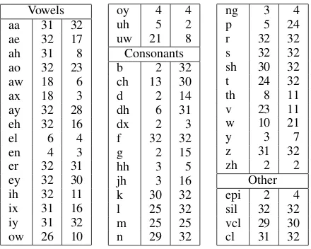
As a final illustration of the nature of the learned models, Table 3 shows the number of substates allo-cated to each phone by the split/merge process (the maximum is 32 for this stage) for the case of hand-aligned (left) as well as automatically-hand-aligned (right) phone boundaries. Interestingly, in the hand-aligned case, the vowels absorb most of the complexity since many consonantal cues are heavily evidenced on adjacent vowels. However, in the automatically-aligned case, many vowel frames with substantial consontant coloring are re-allocated to those adja-cent consonants, giving more complex consonants, but comparatively less complex vowels.

6 Conclusions

We have presented a minimalist, automatic approach for building an accurate acoustic model for phonetic classification and recognition. Our model does not require any a priori phonetic bias or manual spec-ification of structure, but rather induces the struc-ture in an automatic and streamlined fashion. Start-ing from a minimal monophone HMM, we auto-matically learn models that achieve highly compet-itive performance. On the TIMIT phone recogni-tion task our model clearly outperforms standard state-tied triphone models like Young and Wood-land (1994). For phone classification, our model

Vowels

aa 31 32

ae 32 17

ah 31 8

ao 32 23

aw 18 6

ax 18 3

ay 32 28

eh 32 16

el 6 4

en 4 3

er 32 31

ey 32 30

ih 32 11

ix 31 16

iy 31 32

ow 26 10

oy 4 4

uh 5 2

uw 21 8

Consonants

b 2 32

ch 13 30

d 2 14

dh 6 31

dx 2 3

f 32 32

g 2 15

hh 3 5

jh 3 16

k 30 32

l 25 32

m 25 25

n 29 32

ng 3 4

p 5 24

r 32 32

s 32 32

sh 30 32

t 24 32

th 8 11

v 23 11

w 10 21

y 3 7

z 31 32

zh 2 2

Other

epi 2 4

sil 32 32 vcl 29 30

cl 31 32

Table 3: Number of substates allocated per phone. The left column gives the number of substates allocated when training on manually aligned training sequences, while the right column gives the number allocated when we automatically determine phone boundaries.

achieves performance competitive with the state-of-the-art discriminative methods (Sha and Saul, 2006), despite being generative in nature. This result to-gether with our analysis of the context-dependencies and substructures that are being learned, suggests that our model is particularly well suited for mod-eling phone-internal structure. It does, of course remain to be seen if and how these benefits can be scaled to larger systems.

References

P. Clarkson and P. Moreno. 1999. On the use of Sup-port Vector Machines for phonetic classification. In

ICASSP ’99.

S. B. Davis and P. Mermelstein. 1980. Comparison of parametric representation for monosyllabic word recognition in continuously spoken sentences. IEEE Transactions on Acoustics, Speech, and Signal Pro-cessing, 28(4).

J. Glass. 2003. A probabilistic framework for segment-based speech recognition. Computer Speech and Lan-guage, 17(2).

A. Gunawardana, M. Mahajan, A. Acero, and J. Platt. 2005. Hidden Conditional Random Fields for phone recognition. InEurospeech ’05.

A. K. Halberstadt and J. R. Glass. 1998. Hetero-geneous measurements and multiple classifiers for speech recognition. InICSLP ’98.

M. I. Jordan, Z. Ghahramani, T. S. Jaakkola, and L. K. Saul. 1999. An introduction to variational methods for graphical models. Learning in Graphical Models.

L. Lamel and J. Gauvain. 1993. Cross-lingual experi-ments with phone recognition. InICASSP ’93.

K. F. Lee and H. W. Hon. 1989. Speaker-independent phone recognition using Hidden Markov Models.

IEEE Transactions on Acoustics, Speech, and Signal Processing, 37(11).

T. Matsuzaki, Y. Miyao, and J. Tsujii. 2005. Probabilis-tic CFG with latent annotations. InACL ’05.

J. Ming and F.J. Smith. 1998. Improved phone recogni-tion using Bayesian triphone models. InICASSP ’98.

J. J. Odell. 1995. The Use of Context in Large Vocab-ulary Speech Recognition. Ph.D. thesis, University of Cambridge.

S. Petrov, L. Barrett, R. Thibaux, and D. Klein. 2006. Learning accurate, compact, and interpretable tree an-notation. InCOLING-ACL ’06.

L. Rabiner. 1989. A Tutorial on hidden Markov mod-els and selected applications in speech recognition. In

IEEE.

A. Sankar. 1998. Experiments with a Gaussian merging-splitting algorithm for HMM training for speech recognition. InDARPA Speech Recognition Workshop ’98.

F. Sha and L. K. Saul. 2006. Large margin Gaussian mix-ture modeling for phonetic classification and recogni-tion. InICASSP ’06.

N. Ueda, R. Nakano, Z. Ghahramani, and G. E. Hinton. 2000. Split and Merge EM algorithm for mixture mod-els. Neural Computation, 12(9).