Classifier Combination for Contextual Idiom Detection
Without Labelled Data
Linlin Li and Caroline Sporleder Saarland University
Postfach 15 11 50 66041 Saarbr¨ucken
Germany
{linlin,csporled}@coli.uni-saarland.de
Abstract
We propose a novel unsupervised approach for distinguishing literal and non-literal use of idiomatic expressions. Our model com-bines an unsupervised and a supervised classifier. The former bases its decision on the cohesive structure of the context and labels training data for the latter, which can then take a larger feature space into account. We show that a combination of both classi-fiers leads to significant improvements over using the unsupervised classifier alone.
1 Introduction
Idiomatic expressions are abundant in natural lan-guage. They also often behave idiosyncratically and are therefore a significant challenge for natural language processing systems. For example, idioms can violate selectional restrictions (as inpush one’s luck), disobey typical subcategorisation constraints (e.g.,in linewithout a determiner beforeline), or change the default assignments of semantic roles to syntactic categories (e.g., inbreak sth with Xthe argumentXwould typically be an instrument but for the idiombreak the iceit is more likely to fill a patient role, as inbreak the ice with Russia).
In order to deal with such idiosyncracies and as-sign the correct analyses, NLP systems need to be able to recognise idiomatic expressions. Much pre-vious research on idioms has been concerned with
type-based classification, i.e., dividing expressions into ‘idiom’ or ‘not idiom’ irrespective of their ac-tual use in a given context. However, while some expressions, such asby and large, always have an idiomatic meaning, several other expressions, such asbreak the iceorspill the beans, can be used liter-ally as well as idiomaticliter-ally (see examples (1) and (2), respectively). Sometimes the literal usage can even dominate in a domain, as for drop the ball,
which occurs fairly frequently in a literal sense in the sports section of news texts.
(1) Dad had tobreak the iceon the chicken troughs so
that they could get water.
(2) Somehow I always end up spilling the beans all over the floor and looking foolish when the clerk
comes to sweep them up.
Hence, whether a particular occurrence of a po-tentially ambiguous expression has literal or non-literal meaning has to be inferred from the context (token-based idiom classification). Recently, there has been increasing interest in this classification task and both supervised and unsupervised
tech-niques have been proposed. The work we present
here builds on previous research by Sporleder and Li (2009), who describe an unsupervised method that exploits the presence or absence of cohesive ties between the component words of a potential idiom and its context to distinguish between literal and non-literal use. If strong ties can be found the expression is classified as literal otherwise as non-literal. While this approach often works fairly well, it has the disadvantage that it focuses exclu-sively on lexical cohesion, other linguistic cues that might influence the classification decision are disregarded.
We show that it is possible to improve on Sporleder and Li’s (2009) results by employing a two-level strategy, in which a cohesion-based unsupervised classifier is combined with a super-vised classifier. We use the unsupersuper-vised classifier to label a sub-set of the test data with high confi-dence. This sub-set is then passed on as training data to the supervised classifier, which then labels the remainder of the data set. Compared to a fully unsupervised approach, this two-stage method has the advantage that a larger feature set can be ex-ploited. This is beneficial for examples, in which the cohesive ties are relatively weak but which con-tain other linguistic cues for literal or non-literal use.
2 Related Work
Most studies on idiom classification focus on type-based classification; few researchers have worked on token-based approaches (i.e., classification of an expression in a given context). Type-based meth-ods frequently exploit the fact that idioms have a number of properties which differentiate them from other expressions. For example, they often exhibit a degree of syntactic and lexical fixedness. Some idioms, for instance, do not allow internal modi-fiers (*shoot the long breeze) or passivisation (*the
bucket was kicked). They also typically only
al-low very limited lexical variation (*kick the vessel, *strike the bucket).
Many approaches for identifying idioms focus on one of these two aspects. For instance, measures that compute the association strength between the elements of an expression have been employed to determine its degree of compositionality (Lin, 1999; Fazly and Stevenson, 2006) (see also Villav-icencio et al. (2007) for an overview and a com-parison of different measures). Other approaches use Latent Semantic Analysis (LSA) to determine the similarity between a potential idiom and its components (Baldwin et al., 2003). Low similar-ity is supposed to indicate low compositionalsimilar-ity. Bannard (2007) looks at the syntactic fixedness of idiomatic expressions, i.e., how likely they are to take modifiers or be passivised, and compares this to what would be expected based on the ob-served behaviour of the component words. Fazly and Stevenson (2006) combine information about syntactic and lexical fixedness (i.e., estimated de-gree of compositionality) into one measure.
The few token-based approaches include a study by Katz and Giesbrecht (2006), who devise a super-vised method in which they compute the meaning vectors for the literal and non-literal usages of a given expression in the training data. An unseen test instance of the same expression is then labelled by performing a nearest neighbour classification.
Birke and Sarkar (2006) model literal vs. non-literal classification as a word sense disambiguation task and use a clustering algorithm which compares test instances to two automatically constructed seed sets (one with literal and one with non-literal ex-pressions), assigning the label of the closest set. While the seed sets are created without immediate human intervention they do rely on manually cre-ated resources such as databases of known idioms. Cook et al. (2007) and Fazly et al. (2009)
pro-pose an alternative method which crucially relies on the concept ofcanonical form, which is a fixed form (or a small set of those) corresponding to the syntactic pattern(s) in which the idiom normally occurs (Riehemann, 2001).1 The canonical form allows for inflectional variation of the head verb but not for other variations (such as nominal inflection, choice of determiner etc.). It has been observed that if an expression is used idiomatically, it typically occurs in its canonical form. For example, Riehe-mann (2001, p. 34) found that for decomposable idioms 75% of the occurrences are in canonical form, rising to 97% for non-decomposable idioms.2 Cook et al. exploit this behaviour and propose an unsupervised method which classifies an expres-sion as idiomatic if it occurs in canonical form and literal otherwise.
Finally, in earlier work, we proposed an unsu-pervised method which detects the presence or ab-sence of cohesive links between the component words of the idiom and the surrounding discourse (Sporleder and Li, 2009). If such links can be found the expression is classified as ‘literal’ otherwise as ‘non-literal’. In this paper we show that the
per-formance of such a classifier can be significantly improved by complementing it with a second-stage supervised classifier.
3 First Stage: Unsupervised Classifier
As our first-stage classifier, we use the unsuper-vised model proposed by Sporleder and Li (2009). This model exploits the fact that words in a co-herent discourse exhibitlexical cohesion(Halliday
and Hasan, 1976), i.e. concepts referred to in
sen-tences are typically related to other concepts men-tioned elsewhere in the discourse. Given a suitable measure of semantic relatedness, it is possible to compute the strength of such cohesive ties between pairs of words. While the component words of literally used expressions tend to exhibit lexical co-hesion with their context, the words of non-literally used expressions do not. For example, in (3) the ex-pressionplay with fireis used literally and the word
fireis related to surrounding words likegrilling, dry-heat,cooking, andcoals. In (4), howeverplay
with fireis used non-literally and cohesive ties
be-1This is also the form in which an idiom is usually listed in a dictionary.
2Decomposable idioms are expressions such asspill the
beanswhich have a composite meaning whose parts can be mapped to the words of the expression (e.g.,spill→’reveal’,
tweenplayorfireand the context are absent. (3) Grillingoutdoors is much more than just another
dry-heat cooking method. It’s the chance to
play withfire, satisfying a primal urge to stir around incoals.
(4) And PLO chairman Yasser Arafat has accused Israel
ofplaying with fireby supporting HAMAS in its
infancy.
To determine the strength of cohesive links, the unsupervised model builds a graph structure (called
cohesion graph) in which all pairs of content words in the context are connected by an edge which is weighted by the pair’s semantic relatedness. Then theconnectivityof the graph is computed, defined as the average edge weight. If the connectivity increases when the component words of the idiom are removed, then there are no strong cohesive ties between the expression and the context and the example is labelled as ‘non-literal’, otherwise it is labelled as ‘literal’.
To model semantic distance, we use the
Nor-malized Google Distance(NGD, see Cilibrasi and Vitanyi (2007)), which computes relatedness on the basis of page counts returned by a search engine.3 It is defined as follows:
NGD(x, y) = max{log f(x), log f(y)} −log f(x, y) log M−min{log f(x), log f(y)}
(5)
wherexandyare the two words whose association strength is computed (e.g.,fireandcoal),f(x)is the page count returned by the search engine forx (and likewise forf(y)andy),f(x, y)is the page count returned when querying for “x AND y”, and M is the number of web pages indexed by the search engine. The basic idea is that the more often two terms occur together, relative to their overall occurrence, the more closely they are related.
We hypothesise that the unsupervised classifier will give us relatively good results for some exam-ples. For instance, in (3) there are several strong cues which suggest thatplay with fireis used
liter-ally. However, because the unsupervised classifier only looks at lexical cohesion, it misses many other clues which could help distinguish literal and non-literal usages. For example, if break the ice is followed by the prepositionsbetweenoroveras in example (6), it is more likely to be used idiomati-cally (at least in the news domain).
(6) ”Gujral will meet Sharif on Monday and discuss bilateral relations,” the Press Trust of India added.
3We employ Yahoo! rather than Google since we found that it returns more stable counts.
The minister said Sharif and Gujral would be able
to break the ice over Kashmir.
Furthermore, idiomatic usages also exhibit
co-hesion with their context but the cohesive ties are
with thenon-literalmeaning of the expression. For example, in news texts, break the ice in its figu-rative meaning often co-occurs withdiscuss,
rela-tions,talksordiplomacy(see (6)). At the moment we do not have any way to model these cohesive links, as we do not know the non-literal meaning of the idiom.4 However if we had labelled data we could train a supervised classifier to learn these and other contextual clues. The trained classifier might then be able to correctly classify examples which were misclassified by the unsupervised classifier, i.e., examples in which the cohesive ties are weak but where other clues exist which indicate how the expression is used.
For example, in (7) there is weak cohesive evi-dence for a literal use ofbreak the ice, due to the semantic relatedness betweeniceandwater. How-ever, there are stronger cues for non-literal usage, such as the prepositionbetweenand the presence of words likediplomats andtalks, which are in-dicative of idiomatic usage. Examples like this are likely to be misclassified by the unsupervised model; a supervised classifier, on the other hand, has a better chance to pick up on such additional cues and predict the correct label.
(7) Next week the two diplomats will meet in an attempt tobreak the icebetween the two nations. A crucial
issue in the talks will be the long-running water
dispute.
4 Second Stage: Supervised Classifier
For the supervised classifier, we used Support Vec-tor Machines as implemented by the LIBSVM package.5 We implemented four types of features, which encode both cohesive information and word co-occurrence more generally.6
4It might be possible to compute the Normalized Google
Distance between the whole expression and the words in the
context, assuming that whenever the whole expression occurs
it is much more likely to be used figuratively than literally. For expressions in canonical form this is indeed often the case (Riehemann, 2001), however there are exceptions (see
Section 6.1) for which such an approach would not work. 5Available from:http://www.csie.ntu.edu.tw/
˜cjlin/libsvm/We used the default parameters. 6We also experimented with linguistically more informed
features, such as the presence of named entities in the local context of the expression, and properties of the subject or co-ordinated verbs, but we found that these features did not
Salient Words (salW) This feature aims to iden-tify words which are particularlysalientfor literal usage. We used a frequency-based definition of salience and computed theliteral saliency scorefor each word in a five-paragraph context around the target expression:
sallit(w) = loglogf flit(w)×ilit(w)
nonlit(w)×inonlit(w) (8)
wheresallit(w)is the saliency score of the wordw for the classlit;flit(w)is the token frequency of the wordwfor literally used expressions;ilit(w)is the number of instances of the target expressions classified aslitwhich co-occur with wordw(and
mutatis mutandisnonlitfor target expressions la-belled as non-literal).7
Words with a highsallitoccur much more fre-quently with literal usages than with non-literal ones. Conversely, words with a lowsallitshould be more indicative of the non-literal class. How-ever, we found that, in practice, the measure is better at picking out indicative words for the literal class; non-literal usages tend to co-occur with a wide range of words. For example, among the high-est scoring words forbreak the icewe findthick,
bucket, cold, water, reservoiretc. While we do find words likerelations, diplomacy, discussionsamong the lowest scoring terms (i.e., terms indicative of the non-literal class), we also find a lot of noise (ask, month). The effect is even more pronounced for other expressions (like drop the ball) which tend to be used idiomatically in a wider variety of situations (drop the ball on a ban of chemical
weapons,drop the ball on debt reductionetc.). We implement the saliency score in our model by encoding for the 300 highest scoring words whether the word is present in the context of a given exam-ple and how frequently it occurs.8 Note that this feature (as well as the next one) can be computed in a per-idiom or a generic fashion. In the former case, we would encode the top 300 words separately for each idiom in the training set, in the latter across all idioms (with the consequence that more frequent
7Our definition ofsal
litbears similarities with the well knowntf.idfscore. We include both the term frequencies
(flit) and the instance frequencies (ilit) in the formula because
we believe both are important. However, the instance
fre-quency is more informative and less sensitive to noise because
it indicates that expression classified as ’literal’consistently co-occurs with the word in question. Therefore we weight
down the effect of the term frequency by taking itslog. 8We also experimented with different feature dimensions besides 300 but did not find a big difference in performance.
idioms in the training set contribute to more po-sitions in the feature vector). We found that, in practice, it does not make a big difference which variant is used. Moreover, in our bootstrapping scenario, we cannot ensure that we have sufficient examples of each idiom in the training set to train separate classifiers, so we opted for generic models throughout all experiments.
Related Words (relW) This feature set is a vari-ant of the previous one. Here we score the words not based on their saliency but we determine the semantic relatedness between the noun in the id-iomatic expression and each word in the global context, using the Normalized Google Distance
mentioned in Section 3. Again we encode the 300
top-scoring words.
While therelated wordsfeature is less prone to overestimation of accidental co-occurrence than the saliency feature, it has the disadvantage of conflat-ing different word senses. For example, among the highest scoring words foricearecold, melt, snow,
skate, hockeybut alsocream, vanilla, dessert. Relatedness Score (relS) The fourth feature set implements therelatedness scorewhich encodes the scores for the 100 most highly weighted edges in the cohesion graph of an instance.9 If these scores are high, there are many cohesive ties with the surrounding discourse and the target expression is likely to be used literally.
Discourse Connectivity (connect.) Finally, we implemented two features which look at the cohe-sion graph of an instance. We encode the connec-tivity of the graph (i) when the target expression is included and (ii) when it is excluded. The un-supervised classifier uses the difference between these two values to make its prediction. By encod-ing the absolute connectivity values as features we enable the supervised classifier to make use of this information as well.
5 Combining the Classifiers
As mentioned before, we use the unsupervised clas-sifier to label an initial training set for the super-vised one. To ensure that the training set does not contain too much noise, we only add those
ex-amples about which the unsupervised classifier is
9We only used the 100 highest ranked edges because we
are looking at a specific context here rather than the contexts
most confident. We thus need to address two ques-tions: (i) how to define aconfidence functionfor
the unsupervised classifier, and (ii) how to set the confidence thresholdgoverning what proportion of the data set is used for training the second classifier. The first question is relatively easy to answer: as the unsupervised classifier bases its decision on the difference in connectivity between including or excluding the component words of the idiom in the cohesion graph, an obvious choice for a confidence function is the difference in connectivity; i.e., the higher the difference, the higher the confidence of
the classifier in the predicted label.
The confidence threshold could be selected on the basis of the unsupervised classifier’s perfor-mance on a development set. Note that when choos-ing such a threshold there is usually a trade-off be-tween the size of the training set and the amount of noise in it: the lower the threshold, the larger and the noisier the training set. Ideally we would like a reasonably-sized training set which is also rela-tively noise-free, i.e., does not contain too many wrongly labelled examples. One way to achieve this is to start with a relatively small training set and then expand it gradually.
A potential problem for the supervised classifier is that our data set is relatively imbalanced, with the non-literal class being four times as frequent as the literal class. Supervised classifiers often have problems with imbalanced data and tend to be overly biased towards the majority class (see, e.g.,
Japkowicz and Stephen (2002)). To overcome this problem, we experimented with boosting the literal class with additional examples.10 We describe our methods for training set enlargement and boosting the literal class in the remainder of this section. Iteratively Enlarging the Training Set A typi-cal method for increasing the training set is to go through several iterations of enlargement and re-training.11 We adopt a conservative enlargement strategy: we only consider instances on whose la-bels both classifiers agree and we use the confi-dence function of the unsupervised classifier to determine which of these examples to add to the
training set. The motivation for this is that we
hy-pothesise that the supervised classifier will not have
10Throughout this paper, we use the term ’boosting’ in a non-technical sense.
11In our case re-training also involves re-computing the ranked lists of salient and related words. As the process goes on the classifier will be able to discover more and more useful cue words and encode them in the feature vector.
a very good performance initially, as it is trained on a very small data set. As a consequence its con-fidence function may also not be very accurate. On the other hand, we know from Sporleder and Li (2009) that the unsupervised classifier has a rea-sonably good performance. So while we give the supervised classifier a veto-right, we do not allow it to select new training data by itself or overturn classifications made by the unsupervised classifier.
A similar strategy was employed by Ng and Cardie (2003) in a self-training set-up. However, while they use an ensemble of supervised classi-fiers, which they re-train after each iteration, we can only re-train the second classifier; the first one, being unsupervised, will never change its predic-tion. Hence it does not make sense to go through a large number of iterations; the more iterations we go through, the closer the performance of the combined classifier will be to that of the unsuper-vised one because that classifier will label a larger and larger proportion of the data. However, going through one or two iterations allows us to slowly enlarge the training set and thereby gradually im-prove the performance of the supervised classifier. In each iteration, we select 10% of the remain-ing examples to be added to the trainremain-ing set.12 We could simply add those 10% of the data about which the unsupervised classifier is most confident, but if the classifier was more confident about one class than about the other, we would risk obtain-ing a severely imbalanced trainobtain-ing set. Hence, we decided to separate examples classified as ‘literal’ from those classified as ‘non-literal’ and add the top 10% from each set. Provided the automatic classification is reasonably accurate, this will
en-sure that the distribution of classes in the training
set is roughly similar to that in the overall data set
at least at the early stages of the bootstrapping.
Boosting the Literal Class As the process goes
on, we are still likely to introduce more and more
imbalance in the training set. This is due to the fact that the supervised classifier is likely to have some bias towards the majority class (and our ex-periments in Section 6.2 suggest that this is indeed the case). Hence, as the bootstrapping process goes on, potentially more and more examples will be labelled as ’non-literal’ and if we always select the top 10% of these, our training set will gradually
12Since we do not have a separate development set, we
chose the value of 10% intuitively as it seemed a reasonably
become more imbalanced. This is a well-known
problem for bootstrapping approaches (Blum and
Mitchell, 1998; Le et al., 2006). We could coun-teract this by selecting a higher proportion of ex-amples labelled as ’literal’. However given that the number of literal examples in our data set is relatively small, we would soon deplete our literal instance pool and moreover, because we would be forced to add less confidently labelled examples for the literal class, we are likely to introduce more noise in the training set.
A better option is to boost the literal class with external examples. To do this we exploit the fact that non-canonical forms of idioms are highly likely to be used literally. Given that our data set only contains canonical forms (see Section 6.1), we automatically extract non-canonical form variants and label them as ’literal’. To generate possible variants, we either (i) change the number of the noun (e.g.,rock the boatbecomesrock the boats), (ii) change the determiner (e.g.,rock a boat), or (iii) replace the verb or noun by one of its synonyms, hypernyms, or siblings from WordNet (e.g.,rock
the ship). While this strategy does not give us addi-tional literal examples for all idioms, for example we were not able to find non-canonical form occur-rences ofsweep under the carpetin the Gigaword corpus, for most idioms we were able to gener-ate additional examples. Note that this data set is potentially noisy as not all non-canonical form ex-amples are used literally. However, when checking a small sample manually, we found that only very small percentage (<<1%) was mis-labelled.
To reduce the classifier bias when enlarging the training set, we add additional literal examples dur-ing each iteration to ensure that the class distri-bution does not deviate too much from the dis-tribution originally predicted by the unsupervised classifier.13The examples to be added are selected randomly but we try to ensure that each idiom is represented. When reporting the results, we disre-gard these additional external examples.
6 Experiments and Results
We carried out a number of different experiments. In Section 6.2 we investigate the performance of the different features of the supervised classifier and in Section 6.3 we look more closely at the
13We are assuming that the true distribution is not known
and use the predictions of the unsupervised classifier to
ap-proximate the true distribution.
behaviour of the combined classifier. We start by describing the data set.
6.1 Data
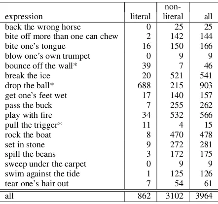
We used the data from Sporleder and Li (2009), which consist of 17 idioms that can be used both literally and non-literally (see Table 1). For each expression, all canonical form occurrences were extracted from the Gigaword corpus together with five paragraphs of context and labelled as ‘literal’ or ‘non-literal’.14 The inter-annotator agreement on a small sample of doubly annotated examples was 97% and the kappa score 0.7 (Cohen, 1960).
non-expression literal literal all
back the wrong horse 0 25 25
bite off more than one can chew 2 142 144
bite one’s tongue 16 150 166
blow one’s own trumpet 0 9 9
bounce off the wall* 39 7 46
break the ice 20 521 541
drop the ball* 688 215 903
get one’s feet wet 17 140 157
pass the buck 7 255 262
play with fire 34 532 566
pull the trigger* 11 4 15
rock the boat 8 470 478
set in stone 9 272 281
spill the beans 3 172 175
sweep under the carpet 0 9 9
swim against the tide 1 125 126
tear one’s hair out 7 54 61
[image:6.595.308.529.245.452.2]all 862 3102 3964
Table 1: Idiom statistics (* indicates expressions for which the literal usage is more common than the non-literal one)
6.2 Feature Analysis for the Supervised Classifier
In a first experiment, we tested the contribution of the different features (Table 2). For each set, we trained a separate classifier and tested it in 10-fold cross-validation mode. We also tested the perfor-mance of the first three features combined (salient and related words and relatedness score) as we wanted to know whether their combination leads to performance gains over the individual classifiers. Moreover, testing these three features in combi-nation allows us to assess the contribution of the connectivity feature, which is most closely related
to the unsupervised classifier. We report the
accu-racy, and because our data are fairly imbalanced,
14The restriction to canonical forms was motivated by the
fact that for the mostly non-decomposable idioms in the set, the vast majority (97%) of non-canonical form occurrences
also the F-Score for the minority class (’literal’). Avg. literal (%) Avg. (%)
Feature Prec. Rec. F-Score Acc.
salW 77.10 56.10 65.00 86.83
relW 78.00 43.20 55.60 84.99
relS 74.90 37.50 50.00 83.68
connectivity 78.30 2.10 4.10 78.58 salW+relW+relS 82.90 63.50 71.90 89.20
all 85.80 66.60 75.00 90.34
Table 2: Performance of different feature sets, 10-fold cross-validation
It can be seen that thesalient words(salW) fea-ture has the highest performance of the individual features, both in terms of accuracy and in terms of
literal F-Score, followed byrelated words(relW),
andrelatedness score(relS). Intuitively, it is plausi-ble that the saliency feature performs quite well as it can also pick up on linguistic indicators of idiom usage that do not have anything to do with lexical cohesion. However, a combination of the first three features leads to an even better performance, sug-gesting that the features do indeed model somewhat different aspects of the data.
The performance of the connectivity feature is also interesting: while it does not perform very well on its own, as it over-predicts the non-literal class, it noticeably increases the performance of the model when combined with the other features, suggesting that it picks up on complementary information.
6.3 Testing the Combined Classifier
We experimented with different variants of the combined classifier. The results are shown in Ta-ble 3. In particular, we looked at: (i) combining the two classifiers without training set enlargement or boosting of the literal class (combined), (ii) boost-ing the literal class with 200 automatically labelled non-canonical form examples (combined+boost), (iii) enlarging the training set by iteration ( com-bined+it), and (iv) enlarging the training set by iteration and boosting the literal class after each iteration (combined+boost+it). The table shows the literal precision, recall and F-Score of the com-bined model (both classifiers) on the complete data set (excluding the extra literal examples). Note that the results for the set-ups involving iterative train-ing set enlargement are optimistic: since we do not have a separate development set, we report the op-timal performance achieved during the first seven
iterations. In a real set-up, when the optimal num-ber of iterations is chosen on the basis of a separate
data set, the results may be lower. The table also shows the majority class baseline (Basemaj), and the overall performance of the unsupervised model (unsup) and the supervised model when trained in
10-fold cross-validation mode (super 10CV). Model Precl Recl F-Scorel Acc.
Basemaj - - - 78.25
unsup. 50.04 69.72 58.26 78.38
combined 83.86 45.82 59.26 86.30
combined+boost 70.26 62.76 66.30 86.13 combined+it∗ 85.68 46.52 60.30 86.68
combined+boost+it∗ 71.86 66.36 69.00 87.03
super. 10CV 85.80 66.60 75.00 90.34
Table 3: Results for different classifiers;∗indicates best performance (optimistic)
It can be seen that the combined classifier is 8% more accurate than both the majority baseline and the unsupervised classifier. This amounts to an error reduction of over 35% (the difference is sta-tistically significant,χ2 test,p << 0.01). While the F-Score of the unboosted combined classifier is comparable to that of the unsupervised one, boost-ing the literal class leads to a 7% increase, due to a significantly increased recall, with no signif-icant drop in accuracy. These results show that
complementing the unsupervised classifier with a
supervised one, can lead to tangible performance gains. Note that the accuracy of the combined clas-sifier, which uses no manually labelled training data, is only 4% below that of a fully supervised classifier; in other words, we do not lose much by starting with an automatically labelled data set.
It-erative enlargement of the training set can lead to
further improvements, especially when combined with boosting to reduce the classifier bias.
To get a better idea of the effect of training set enlargement, we plotted the accuracy and F-Score of the combined classifier for a given number of iterations with boosting (Figure 1) and without (Fig-ure 2). It can be seen that enlargement has a notice-able positive effect if combined with boosting. If
the literal class is not boosted, the increasing bias
of the classifier seems to outweigh most of the pos-itive effects from the enlarged training set. Figure 1 also shows that the best performance is obtained af-ter a relatively small number of iaf-terations (namely two), as expected.15 With more iterations the per-formance decreases again. However, it decays
rel-15Note that this also depends on the confidence threshold.
For example, if a threshold of 5% is chosen, more iterations
atively gracefully and even after seven iterations, when more than 40% of the data are classified by the unsupervised classifier, the combined classifier still achieves an overall performance that is sig-nificantly above that of the unsupervised classifier (84.28% accuracy compared to 78.38%, significant at p << 0.01). Hence, the combined classifier seems not to be very sensitive to the exact number of iterations and performs reasonably well even if the number of iterations is sub-optimal.
1 2 3 4 5 6 7
Iterations
50 50
55 55
60 60
65 65
70 70
75 75
80 80
85 85
90 90
95 95
Performance
[image:8.595.305.519.122.280.2]Acc. combined Acc. unsupervised F-Score combined F-Score unsupervised
Figure 1: Accuracy and literal F-Score on complete data set after different iterations with boosting of the literal class
1 2 3 4 5 6 7
Iteration
50 50
55 55
60 60
65 65
70 70
75 75
80 80
85 85
90 90
95 95
Performance
2 4 6
[image:8.595.73.290.203.359.2]Acc. combined Acc. unsupervised F-Score combined F-Score unsupervised
Figure 2: Accuracy and literal F-Score on complete
data set after different iterations without boosting of the literal class
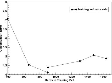
Figure 3 shows how the training set increases as the process goes on16 and how the number of mis-classifications in the training set develops. In-terestingly, when going from the first to the second iteration the training set nearly doubles (from 396
to 669 instances), while the proportion of errors is also reduced by a third (from 7% to 5%). Hence, the training set does not only grow but the pro-portion of noise in it decreases, too. This shows
16Again, we disregard the extra literal examples here.
that our conservative enlargement strategy is fairly successful in selecting correctly labelled examples. Only at later stages, when the classifier bias takes over, does the proportion of noise increase again.
400 600 800 1000 1200 1400 1600
Items in Training Set 4
4.5 5 5.5 6 6.5 7 7.5 8
Classification Error
training set error rate
Figure 3: Training set size and error in training set at different iterations
7 Conclusion
We presented a two-stage classification approach for distinguishing literal and non-literal use of id-iomatic expressions. Our approach complements an unsupervised classifier, which exploits informa-tion about the cohesive structure of the discourse, with a supervised classifier. The latter can make use of a range of features and therefore base its classification decision on additional properties of the discourse, besides lexical cohesion. We showed that such a combined classifier can lead to a sig-nificant reduction of classification errors. Its per-formance can be improved further by iteratively increasing the training set in a bootstrapping loop and by adding additional examples of the literal class, which is typically the minority class. We found that such examples can be obtained automat-ically by extracting non-canonical variants of the target idioms from an unlabelled corpus.
Future work should look at improving the su-pervised classifier, which so far has an accuracy of 90%. While this is already pretty good, a more sophisticated model might lead to further improve-ments. For example, one could experiment with linguistically more informed features. While our initial studies in this direction were negative, care-ful feature engineering might lead to better results.
Acknowledgements
This work was funded by the Cluster of Excellence
[image:8.595.73.291.418.572.2]References
Timothy Baldwin, Colin Bannard, Takaaki Tanaka, and Dominic Widdows. 2003. An empirical model of multiword expression decomposability. In Proceed-ings of the ACL 2003 Workshop on Multiword Ex-pressions: Analysis, Acquisition and Treatment.
Colin Bannard. 2007. A measure of syntactic flibility for automatically identifying multiword ex-pressions in corpora. InProceedings of the ACL-07 Workshop on A Broader Perspective on Multiword Expressions.
Julia Birke and Anoop Sarkar. 2006. A clustering approach for the nearly unsupervised recognition of nonliteral language. InProceedings of EACL-06.
Avrim Blum and Tom Mitchell. 1998. Combining la-beled and unlala-beled data with co-training. In Pro-ceedings of COLT-98.
Rudi L. Cilibrasi and Paul M.B. Vitanyi. 2007. The Google similarity distance. IEEE Trans. Knowledge and Data Engineering, 19(3):370–383.
Jacob Cohen. 1960. A coefficient of agreement for nominal scales. Educational and Psychological Measurements, 20:37–46.
Paul Cook, Afsaneh Fazly, and Suzanne Stevenson. 2007. Pulling their weight: Exploiting syntactic forms for the automatic identification of idiomatic expressions in context. InProceedings of the ACL-07 Workshop on A Broader Perspective on Multi-word Expressions.
Afsaneh Fazly and Suzanne Stevenson. 2006. Auto-matically constructing a lexicon of verb phrase id-iomatic combinations. InProceedings of EACL-06.
Afsaneh Fazly, Paul Cook, and Suzanne Stevenson. 2009. Unsupervised type and token identification of idiomatic expressions. Computational Linguistics, 35(1):61–103.
M.A.K. Halliday and R. Hasan. 1976. Cohesion in English. Longman House, New York.
Nathalie Japkowicz and Shaju Stephen. 2002. The class imbalance problem: A systematic study. In-telligent Data Analysis Journal, 6(5):429–450.
Graham Katz and Eugenie Giesbrecht. 2006. Au-tomatic identification of non-compositional multi-word expressions using latent semantic analysis. In
Proceedings of the ACL/COLING-06 Workshop on Multiword Expressions: Identifying and Exploiting Underlying Properties.
Anh-Cuong Le, Akira Shimazu, and Le-Minh Nguyen. 2006. Investigating problems of semi-supervised learning for word sense disambiguation. In Proc. ICCPOL-06.
Dekang Lin. 1999. Automatic identification of non-compositional phrases. InProceedings of ACL-99, pages 317–324.
Vincent Ng and Claire Cardie. 2003. Weakly super-vised natural language learning without redundant views. InProc. of HLT-NAACL-03.
Susanne Riehemann. 2001. A Constructional Ap-proach to Idioms and Word Formation. Ph.D. thesis, Stanford University.
Caroline Sporleder and Linlin Li. 2009. Unsupervised recognition of literal and non-literal use of idiomatic expressions. InProceedings of EACL-09.