Realization of the Linear Tree that Corresponds to a Fundamental Loop Matrix

doi:10.4236/wsn.2010.21004Published Online January 2010 (http://www.SciRP.org/journal/wsn/).

Realization of the Linear Tree that Corresponds to a

Fundamental Loop Matrix

Jianping QIAN1, Peng-Yung WOO2

1

Department of Automation, Nanjing University of Science and Technology, Nanjing, China

2

Department of Electrical Engineering, Northern Illinois University, Dekalb, USA Email: pwoo@niu.edu

Received October 13, 2009; revised October 27, 2009; accepted October 28, 2009

Abstract

Graph realization from a matrix is an important topic in network topology. This paper presents an algorithm for the realization of a linear tree based on the study of the properties of the number of the single-link loops that are incident to each tree branch in the fundamental loop matrix Bf. The proposed method judges the

pendent properties of the tree branches, determines their order one by one and then achieves the realization of the linear tree. The graph that corresponds to Bf is eventually constructed by adding links to the obtained

linear tree. The proposed method can be extended for the realization of a general tree.

Keywords:Fundamental Loop Matrix, Linear Tree, Graph

1. Introduction

Graph realization from a matrix is an important topic in network topology. It has a broad application in electrical networks, switching networks, linear programming etc. The study of graph realization from a matrix is to judge whether a given matrix can be realized to be a graph. If yes, the method for realization needs to be found so that graph realization for a given matrix can be achieved. There are three aspects in graph realization from a matrix: a) the realizablity of the given matrix, b) the method for graph realization from a matrix, c) the unique corre-spondence between the realized graph and the given ma-trix. All the above issues have been under research by using algebra theory, graph theory, geometry structure etc [1–5]. While the necessary and sufficient conditions for the realizability of a graph from a matrix are pro-posed by many researchers from different viewpoints, the judgment of the realizability and the realization of the graph, in practice, are carried out simultaneously rather than in sequence.

Quite a few researchers studied the realization of a linear tree [6,7]. This paper presents an algorithm for the realization of a linear tree based on the study of the properties of the number of the single-link loops that are incident to each tree branch in the fundamental loop ma-trix Bf. The proposed method judges the pendent

proper-ties of the tree branches, determines their order one by one and then achieves the realization of the linear tree.

Since a general tree possesses a linear sub-tree, a general tree can then be realized by adding other tree branches after the linear sub-tree is realized. The graph that corre-sponds to an arbitrary fundamental loop matrix Bf is

eventually constructed by adding links to the obtained linear tree. As is seen, the proposed method is simple, practical and efficient in realizing a general tree.

2. Pretreatment

For a graph that possesses n nodes and b branches, after a certain tree T is chosen, the fundamental loop matrix Bf

has a standard form [Bt 1] where Bt is a (b-n+1)(n-1)

matrix. Assume that the columns b1, b2, …, bn-1 in Bt

  



our discussions, it is assumed that the tree that corre-sponds to Bt is a linear tree. For example:

1 2 3 4 5 6 4 1 1 1 1 0 0 [ , ] 5 1 1 0 0 1 0 6 0 1 1 0 0 1

 

 

 



B B 1

f t

The number of the pairs of corresponding entries be-ing all “1”s in b1 and b2 (i.e., row 1 and row 2) is 2. Thus,

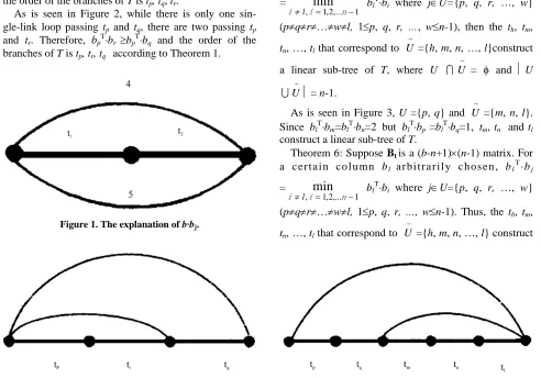
b1Tb2=2. By realizing a graph (Figure 1) from the matrix

that is constructed by the rows of the

aforementioned pairs as well as the same indexed rows in the corresponding link columns, we know that b1Tb2=2 is the number of the single-link loops that pass t1 and t2. Specially, b1Tb1=2 is the number of the single-link loops that pass t1. The following theorems present the rela-tionship among the branches of T (Due to limitation of space, the proofs are not presented in this article).

1 2 4 5 4 1 1 1 0 5 1 1 0 1



 

 

Theorem 1: Suppose Bt is a (b-n+1)3 matrix and tpis a pendent branch of the linear tree T that corresponds to

Bt. If and only if bpTbqbpTbr(pqr, p, q, r=1, 2, 3), the order of the branches of T is tp, tq, tr.

As is seen in Figure 2, while there is only one sin-gle-link loop passing tp and tq, there are two passing tp and tr. Therefore, bpTbr bpTbq and the order of the branches of T is tp, tr, tq according to Theorem 1.

Figure 1. The explanation of b·bj.

Figure 2. The explanation of Theorem 1.

Theorem 2: Suppose Bt is a (b-n+1)(n-1) matrix and

tp is a pendent branch of the linear tree T that corre-sponds to Bt. If and only if bpTbqbpTbr (pqr, 1p, q,

rn-1), the order of the branches of T is tp, …, tq, …, tr (i.e., tq is closer to tpthan tr is).

Theorem 3: Suppose Bt is a (b-n+1)(n-1) matrix. For

a certain column bl arbitrarily chosen, if blTbp

= blTbi (pl, 1pn-1), tp is a pendent

branch of the linear tree T that corresponds to Bt.

min

1 ,... 2 , 1

,  

 i n

i

l

Theorem 4: Suppose Bt is a (b-n+1)(n-1) matrix. For

a certain column bl arbitrarily chosen, if blTbj

= blTbi where jU={p, q, r, …, w}

(pqr…wl, 1p, q, r,…, wn-1), there must exist a certain sU such that ts is a pendent branch of the linear tree T that corresponds to Bt.

min

1 ,... 2 , 1

,  

 i n

i

l

As is seen in Figure 3, while blTbm=blTbn=2, blTbp =blTbq=1. Thus, there must exist a certain sU={p, q} such that tpor tq is a pendent branch of the linear tree T.

Theorem 5: Suppose Btis a (b-n+1)(n-1) matrix. For

a certain column bl arbitrarily chosen, if blTbj

= blTbi where jU={p, q, r, …, w}

(pqr…wl, 1p, q, r, …, wn-1), then the th, tm,

tn, …, tl that correspond to ={h, m, n, …, l}construct

a linear sub-tree of T, where U =  and U

= n-1.

min

1 ,... 2 , 1

,  

 i n

i

l

U



U

 U

As is seen in Figure 3, U ={p, q} and ={m, n, l}. Since blTbm=blTbn=2 but blTbp=blTbq=1, tm,tn andtl construct a linear sub-tree of T.

 U

Theorem 6: Suppose Btis a (b-n+1)(n-1) matrix. For

a c e r t a i n c o l u mn bl a r b i t r a r i l y c h o s e n , blTbj

= blTbi where jU={p, q, r, …, w}

(pqr…wl, 1p, q, r,…, wn-1). Thus, the th, tm,

tn, …, tl that correspond to ={h, m, n, …, l} construct

min

1 ,... 2 , 1

,  

 i n

i

l



U

a linear sub-tree of T, where U =  andU

= n-1. Then for a certain k , if there are

cer-tain s1 and s2U*U such that , after

the links L’s that correspond to in

the graph G that corresponds to Bf are deleted, the graph

constructed by G1 that corresponds to U* and the graph G2 that corresponds to (U-U*)



is a separable graph, where G1 and G2G, G1G2GL=G, G1 G2GL= and GL is the graph that corresponds to the links L’s. If G1 and G2 are inseparable graphs, respectively, then G1 and G2 have a common cut-point.

 

U

1 s

b

max

m, h,



U

b



n,..., U

2 s T k T

k b

b 

l

k

T k

b 

U

 

1 s

b

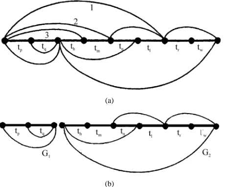
As is seen in Figure 4(a), blTbj =1 where jU={p, q, r,

w}. Thus, theth, tm, tn, …, tl that correspond to



U={h, m,

n, l}construct a linear sub-tree of T. Let k=h  U

2

, and s1

and s2U*={p, q}U. Since =3, links

1, 2 and 3 are deleted. The remaining G1 and G2 are separable graphs as shown in Figure 4(b).

1 T k s T

k b b b

b    _s

From the above facts, it is seen that when the condi-tions in Theorem 6 are satisfied, G1 and G2 are 2-iso-morphic. Therefore, in the ordering of the branches of the linear tree, the branches of the linear sub-tree that corresponds to G1 are first put into order separately, then those of the linear sub-tree that corresponds to G2. The ordering of the branches of the linear tree is now reduced to the ordering of the branches for each linear sub-tree. The solution of this problem is depending on the follow-ing Theorem 7, where it is assumed that the sub-trees do not form 2-isomorphism.

(a)

(b)

Figure 4. The explanation of Theorem 6.

Theorem 7: Suppose Btis a (b-n+1)(n-1) matrix. For

a certain column bl arbitrarily chosen, blTbj

= blTbi where jU={p, q, r, …,

w}(pqr…wl, 1p, q, r,…, wn-1). Thus, the th, tm,

tn, …, tl that correspond to ={h, m, n, …, l}construct

a linear sub-tree of T, where U = and U

=n-1. Then for a certain k , if there is a certain

sU such that = , is a

pendent branch of the linear tree T that corresponds to Bt.

min

1 ,... 2 , 1

,  

 i n

i

l



U

T k

b 



U

min

p, j



w 

U

T k

b

 U

r,..., q,

s

b s,

j j

b



_t

As is seen in Figure 5, U={p, q, r} and ={h, m, n,

l}. Let k=h and s=pU. Since

and , is a pendent branch of

the linear tree T.



U

1  

U

1 

2  

 T _q

h p T

h b b b

b

3   

 T _r

h p T

h b b b

b t_p

3. The Algorithm for the Construction of the

Linear Tree

We propose the following algorithm for the construction of the linear tree T. The thread of thinking is that one of the two pendent branches of T, e.g., tpis foundfirst. The other pendent tree branch tq is found by using tp as a base. Then tq is taken off, the other pendent tree branch tr is found by using tp as a base again. Keep on with this pro-cedure until the order of all the branches of T is decided. 1) For a given fundamental loop matrix Bf=[Bt 1], let

M=BtTBt where the entry = . Establish a

ma-trix Bt’ which is of the same dimension as Bt so that the

columns of Bt after ordering can be put into Bt’. Let the

column index for Bt’ be f. Set f=1.

ij

m

T

2) For row i (1in-1) in M (Usually, let i=1 first to follow the row order in M), if there is only one entry mip in row i that takes the minimum value, tp that corre-sponds to column p is a pendent branch of the linear tree

T according to Theorem 3. Go to step (6). On the other hand, if there are multiple entries , , , …,

in row i that take the minimum value, there must

exist a certain sUd={pd, qd, rd, …, wd} (d is the iteration index. Let d=1 first.) such that tsthat corresponds to column s is a pendent branch of the linear tree T

accord-d ip m d iq m d ir m d iw m

ing to Theorem 4.

3) For row k in M where k ={h, m, n, …,

l}(Usually, let k follow the row order in ), if there is only one entry mks in row k thattakes the minimum value where sUd, tsthat corresponds to column s is a pendent branch of the linear tree T according to Theorem 7.

d U  d U  Go to step (4). On the other hand, if there are multiple en-tries , , , …, in row k that take

the minimum value, there must exist a certain sUd={pd,

qd, rd, …, wd} (d=d+1) such that tsthat corresponds to column s is a pendent branch of the linear tree T

accord-d kp m d kq m d kr m d kw m

ing to Theorem 4. Repeat step (3) until k takes all the

elements in . At that time, if there are still multiple entries in row k that take the minimum value, go to step (8).

d

U



4) If the last column of Bt’ is not filled by a column

from Bt yet, set p=s. Go to step (6). Otherwise, judge the

adjacency of tk, ts and tp according to Theorem 2.

5) If tk and tp are at the same side of ts, i.e., the order is ts, …, tk, …, tp, set p=s. Go to step (6). On the other hand, if tk and tp are at the different sides of ts, i.e., the order is tk, …, ts, …, tp, use tk as a pendent tree branch to find the order of the tree branches corresponding to Ud and put them into the columns of Bt’, i.e., column f

to column f’ where f’=f+(number of elements in Ud)-1. Set all the entries in the columns of M corresponding to Ud to be . If the entries in M are all , stop. If not, set f = f+ (number of elements in Ud). Go back to step (2).

6) If the last column of Bt’ is already filled by a

col-umn from Bt, i.e., a pendent tree branch at one end is

already decided, go to step (b). Otherwise

a) Assume the pendent branch of T is tp. Put tp into the last column of Bt’. Set i=p. Go to step (7).

b) Put column p of Btinto column f of Bt’. Set f=f+1.

7) If all the columns of Bt have been put into Bt’, the

ordered columns of Bt’ have already constitute a linear

tree. Stop. Otherwise, set the entries in column p of M to be . Go back to step (2).

8) When there are only two entries in Ud, choose ar-bitrarily sUd. ts is a pendent branch of T. Go to step (4). Otherwise, according to Theorem 5 and Theorem 6, the linear sub-tree in graph G1 that corresponds to

Ud*=Udcan be put into order separately. Thus, take the columns Bt(1) in Bt that correspond to the elements in

Ud to construct Bt(1)T Bt(1)=M(1). Repeat steps (2)-(8)

for M(1). If the number of elements in Ud is not changed after one iteration, the order of the corre-sponding tree branches is arbitrary. Put the ordered columns of Bt(1) into column f to column f’ where

f’=f+(number of elements in Ud)-1. Set all the entries in the columns of M corresponding to Ud to be . If the entries in M are all , stop. If not, set f=f+(number of elements in Ud). Go back to step (2).

4. An Example

Given a fundamental loop matrix

Br= ,

            1 0 0 0 1 1 1 0 0 0 1 0 0 1 0 1 1 1 0 0 1 0 1 0 0 0 1 0 0 0 1 1 1 1 1 1 9 8 7 6 5 4 3 2 1 we have

Bt = and BtT .

            1 1 1 0 0 1 0 1 1 1 1 0 0 0 1 1 1 1 1 1 5 4 3 2 1                  1 1 1 1 1 0 0 1 1 1 0 1 0 1 0 1 0 1 1 1

a) According to step (1),

M=BtTBt= .

                4 2 3 2 3 2 2 2 1 1 3 2 3 2 2 2 1 2 2 2 3 1 2 2 3 5 4 3 2 1 5 4 3 2 1

Also, establish a matrix Bt’ which is of the same

di-mension as Bt so that the columns of Bt after ordering

can be put into Bt’. Let the column index for Bt’ be f. Set

f=1.

b) According to step (2), consider row 1 of M. As m14 is the only entry in row 1 that takes the minimum value, t4 is one pendent branch of T. Go to step (6).

c) According to step (6)(a), put column 4 of Bt into the

last column of Bt’, i.e.,

Bt’= . Set i=4.

d) According to step (7), set all the entries in column 4 of M to be , i.e.,

M =

                     4 3 2 3 2 2 1 1 3 3 2 2 2 2 2 2 3 2 2 3 5 4 3 2 1 5 4 3 2 1

e) According to step (2), consider row 4 of M. As m41 andm42 are the entries in row 4 that take the minimum value, there must exist the other pendent branch of T among t1 and t2 that correspond to U1={1, 2}. Here,

={3, 4, 5}. 1



U

f) According to step (3), consider row 3 of M. As m31 andm32 are the entries in row 3 that take the minimum value, there must exist the other pendent branch of T among t1 and t2 that correspond to U2={1, 2}. Here,

={3, 4, 5}. 2



U

g) Repeat step (3). Consider row 5 of M. m52 is the only entry in row 5 that takes the minimum value.

h) According to step (4), as the last column of Bt’ is

already filled by a column from Bt, judge the adjacency

of t5, t2 and t4. As m42<m45 in m4, the order is t2, …,

t5, …, t4.

i) According to step (5), as t5 and t4 are at the same side of t2, t2 is the other pendent branch of T that is based on t4. Set p=2.

j) According to step (6)(b), put column 2 of Bt into the

first column of Bt’, i.e., Bt’= . Set

f=1+1=2.             1 0 0 1 0 0 1 1 4 2

k) According to step (7), set all the entries in column 2 of M to be , i.e.,

M = .

                          4 3 3 2 2 1 3 3 2 2 2 2 3 2 3 5 4 3 2 1 5 4 3 2 1

l) According to step (2), consider row 4 of M. As m41 is the only entry in row 4 that takes the minimum value, t1 is the other pendent branch of T that is based on t4 with

t2 taken off.

m) According to step (6), put column 1 of Bt into the

second column of Bt’, i.e., Bt’= . Set

f=2+1=3.             1 0 0 0 1 1 0 1 0 1 1 1 4 1 2

n) According to step (7), set all the entries in column 1 of M to be , i.e.,

M = .

                               4 3 2 2 3 3 2 2 3 2 5 4 3 2 1 5 4 3 2 1

o) According to step (2), consider row 4 of M. As m43 andm45 are the entries in row 4 that take the minimum value, there must exist the other pendent branch of T that is based on t4with t1 and t2 taken off among t3and t5that

correspond to U1={3, 5}. Here, U1={1, 2, 4}.



p) According to step (3), consider row 1 of M. m13 is the only entry in row 1 that takes the minimum value.

q) According to step (4), as the last column of Bt’ is

already filled by a column from Bt, judge the adjacency

of t1, t3 and t4. As m13>m14in m1, the order is t1, …, t3, …,

t4.

r) According to step (5), as t1 and t4 are at the different sides of t3, t2 is used as the other pendent branch of T to find the order of the tree branches corresponding to Ud. Put column 3 of Bt into the fourth (f’=3+2-1=4) column

of Bt’, i.e.,

Bt’= .

            1 1 0 0 0 1 1 1 0 0 1 0 1 1 1 1 4 3 1 2

Set f=3+1=4. Set all the entries in column 3 of M to be , i.e.,

M = .

                                    4 2 3 2 3 5 4 3 2 1 5 4 3 2 1

5. Conclusions

t3 taken off.

t) According to step (6), put column 5 of Bt into the

third column of Bt’, i.e., Bt’= . Set

f=4+1=5.

   

 

   

 

1 1 1 0 0

0 1 1 1 1

0 0 1 1 0

1 1 1 1 1

4 3 5 1

2 _{This paper presents an algorithm for the realization of a}

linear tree based on the judgment of the pendent proper-ties of the tree branches and the determination of their order one by one. The graph that corresponds to Bf is

eventually constructed by adding links to the obtained linear tree. As an arbitrary tree contains a linear tree, the linear tree can then be realized first to realize a general tree. This will be discussed in another paper of ours. u) According to step (7), stop.

The main contribution of this paper lies in the proposi-tion of a new approach to the realizaproposi-tion of a linear tree. Experiments validate the effectiveness of the proposed approach. This lays a foundation to the realization of a general tree and therefore a random graph from a given matrix.

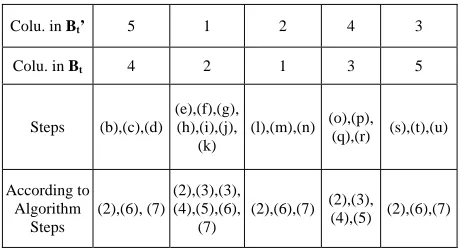
As a summary, we have the following table to achieve the order of the columns in Bt’.

Colu. in Bt’ 5 1 2 4 3

Colu. in Bt 4 2 1 3 5

Steps (b),(c),(d) (e),(f),(g), (h),(i),(j),

(k)

(l),(m),(n) (o),(p),

(q),(r) (s),(t),(u)

According to Algorithm

Steps

(2),(6), (7)

(2),(3),(3), (4),(5),(6),

(7)

(2),(6),(7) (2),(3),

(4),(5) (2),(6),(7)

6. References

[1] L. Q. Lei and B. Q. Dai, “A convenient method for for-mulation of a node incidence matrix from a basic cutset matrix,” (In Chinese), Journal of Jiangxi Polytechnic University, Vol. 14, No. 3, September 1992.

[2] W. Mayeda, “Graph theory,” John Wiley, New York, 1972.

The column order [2, 1, 5, 3, 4] of Bt’ is thus the

or-der of the branches of the linear tree as shown by the bold segments in Figure 6. The graph that corresponds to Bf can then be obtained by adding the links 6, 7, 8

and 9.

[3] K. P. Rajappan, “On Okada’s method for realizing cutset matrices,” Journal of Combinational Theory, Vol. 10, pp. 135–142, 1971.

[4] M. N. S. Swamy and K. Thulasiraman, “Graph, network and algorithms,” John Wiley, New York, 1981.

[5] L. Zhu, “An expression for the relationship between the incidence Matrix A of Graph G and the basic loop Matrix Bf,” (In Chinese), Teaching and Scientific Technology, No. 1, pp. 72–75, March 1996.

[6] R. B. Ash and W. H. Kim, “On realizability of a circuit matrix,” IRE Transactions on Circuit Theory, Vol. CT-6, pp. 219–223, June 1959.

[7] S. R. Parker and H. J. Lohse, “A direct procedure for the synthesis of network graphs from a given fundamental loop or cutset matrix,” IEEE Transactions on Circuit The-ory, Vol. CT-16, pp. 221–223, May 1969.