Coagulation equations with mass loss
Jonathan AD Wattis
†, D Graham McCartney
‡& Throstur Gudmundsson
§†Theoretical Mechanics, School of Mathematical Sciences,
University of Nottingham, University Park, Nottingham, NG7 2RD, U.K. ‡ School of Mechanical, Materials, Manufacturing Engineering and Management,
University of Nottingham, University Park, Nottingham, NG7 2RD, U.K. § VST Engineers, Armula 4, 108 Reykjavik, Iceland.
email: [email protected] [email protected]
August 2003
Abstract
We derive and solve models for coagulation with mass loss arising, for example, from industrial processes in which growing inclusions are lost from the melt by colliding with the wall of the vessel. We consider a variety of loss laws and a variety of coagulation kernels, deriving exact results where possible, and more generally reducing the equations to similarity solutions valid in the large-time limit. One notable result is the effect that mass removal has on gelation: for small loss rates, gelation is delayed, whilst above a critical threshold, gelation is completely prevented. Finally, by forming an exact explicit solution for a more general initial cluster size distribution function, we illustrate how numerical results from earlier work can be interpreted in the light of the theory presented herein.
Keywords: Smoluchowski coagulation, aggregation, cluster size distribution.
1
Introduction
Aluminium and its alloys are of increasing importance in many industrial sectors for packaging, transport and construction uses. In recent years, there has been a growing recognition that in many applications material performance is limited by the presence of micrometre-sized, insoluble inclusions that are introduced into the molten metal by melting and refining processes which are conducted prior to the casting of ingots or components, for examples see Engh [1] and Simensen [2]. Critical properties of, for example, ultra thin foil and thin strip for the packaging industry can be adversely affected by the presence of such non-metallic inclusions.
In the production of aluminium alloys, molten metal is held in a furnace for periods of up to several hours before it is cast. At this stage, sub-micrometre sized particles of the insoluble, high melting point chemical compound titanium diboride (TiB2) are added for the purpose of efficiently
nucleating solid aluminium during subsequent solidification and casting (McCartney [3]). However, whilst holding the melt in the furnace these TiB2 particles can both agglomerate and also be lost
the capability to measure inclusion content and size distribution in molten aluminium, for example see Martin [4], there is still a lack of understanding of the kinetics of coagulation in this system. It is in this context that the present study was undertaken.
Over recent years, generalised forms of Smoluchowski’s coagulation equations have been devel-oped to model the size-evolution of clusters of particles in such systems. Leyvraz & Tschudi [5] have noted that the coagulation equations without mass loss could be solved exactly if the coagulation rates were given by one of two special kernels, that is a function which specifies how the rate of coagulation depends on the size of the aggregating clusters. The solvable cases which they describe are the size-independent kernel ai,j =aand the size-dependent kernel ai,j =a(i+j). Our approach
originally outlined in Davieset al.[6] uses generating functions, and delivers explicit solutions more simply. This method has been extended to model situations with mass addition (Davies et al. [7]) and mass loss through direct interaction between clusters and the gel (Wattis et al. [8]).
Singh & Rodgers [9] considered aggregation processes which occur simultaneously with mass loss in the framework of a continuous model. They consider the scenario where oxidation, melting or evaporation occur on the exposed surface of clusters, and hence take the mass loss term to have the form −∂
∂j(m(j)c(j, t)), where c(j, t) or cj(t) denotes the concentration of clusters of size j at
time t. Hendriks [10] also considers aggregation with mass loss, but only when the aggregation kernel has the form ai,j =aij, this is the classic kernel which allows gelation and an exact explicit
solution in the case of pure coagulation. The mass loss term used by Hendricks has a similar form to that used by us, namely, Lj = Acj +Bjcj in the notation introduced later on. Finally we
should note the work of Rotstein et al.[11] in which a mass loss term is introduced in the monomer equation. In a similar way to the more general loss term we consider, their term can delay or totally prevent gelation in the case of the coagulation kernel which permits gelation to occur, and they analyse how the amount of gel formed depends on the strength of the rate of mass removal.
1.1
Model
We useCkto denote a cluster composed ofkmonomers. The kinetics of the standard Smoluchowski
agglomeration process
Ci+Cj →Ci+j, rate =ai,j (1.1)
with aggregation rate ai,j can be modelled by defining the concentration of Cj to be cj(t). Using
the law of mass action we then obtain
dcj(t)
dt =
1 2
j−1
X
i=1
ai,j−ici(t)cj−i(t)− ∞
X
i=1
ai,jci(t)cj(t). (1.2)
Deriving the second sum is more straightforward than the first, it comes from the fact that a cluster
Cj can combine with a cluster Ci of any size 1 ≤i < ∞ as described by (1.1). Thus we sum over
all i to obtain the rate at which Cj clusters are lost due to aggregation. The first sum in (1.2)
comes from the rate at which Cj clusters are created by the coalescence of smaller clusters through
Ci +Cj−i → Cj. The factor of one half is present to prevent double counting of this process.
Since matter is neither created or destroyed in the coagulation process we expect the total number of monomers in the system M1 = P
∞
j=1jcj to be time-independent. As a check of (1.2), M1 can
be shown formally to be a constant. More details about this calculation are given at the start of Section 2.3. To the standard Smoluchowski coagulation equations (1.2) we add a mass loss term of the form Cj →φ with rate Lj(cj), hence we obtain the system of equations
dcj(t)
dt =
1 2
j−1
X
i=1
ai,j−ici(t)cj−i(t)− ∞
X
i=1
In the model of interest to Gudmundsson [12] the clusters are micrometre-sized nonmetallic inclusions (TiB2) in molten aluminium and the aggregation rates are determined by ai,j = (Ri+
Rj)(Di +Dj). Here Ri is the radius of a sphere with volume iV0 for some element of volume V0,
thus Ri ∝i1/3; and Di is the corresponding diffusion constant, with Di ∝1/Ri. This corresponds
to the continuum regime of Brownian coagulation. Many other kernels have been used to model aggregation processes, see da Costa [13] for examples. In the process analysed by Gudmundsson, mass is lost by removal of particles from the melt by transfer to the walls of the holding furnace for the molten metal. This occurs at a rate Lj(cj(t)) =Ljλcj(t) for some L and λ = 2/3.
We shall consider a more general problem, in which λis not constrained to 2/3, but could take any value, and in which the coagulation kernel has the form ai,j =aiαjα(iβ+jβ). This covers the
integrable cases ai,j =a(α=β = 0), as well asai,j =a(i+j) (α = 0,β = 1), andai,j =aij (α = 1,
β = 0). The Brownian kernel of Gudmundsson corresponds to a combination of the constant kernel
ai,j =a and the case α=−1/3, β = 2/3.
We thus have the system of equations
dcj(t)
dt =
1 2
j−1
X
i=1
ai,j−ici(t)cj−i(t)− ∞
X
i=1
ai,jci(t)cj(t)−Ljλcj(t), (1.4)
which models the simultaneous aggregation and mass loss processes. It is the presence of a mass loss term which is novel in the current study of the coagulation equations. We describe cases in which information about the solution can be derived exactly and explicitly; this corresponds to the case λ = 0, where the generating function approach yields a complete solution. The existence of a closed form exact solution to such a complicated system of equations is remarkable, and the solution forλ >0 will share many properties of the solution forλ= 0. We then examine the case of general λ in more detail, by use of large-time asymptotic methods, and by assuming the existence of a self-similar solution, which enables various scaling behaviours of the solution to be elucidated. In the analysis of gelation in a truncated version of Smoluchowski’s coagulation equations, da Costa derived an equation of the form (1.4), namely equation (10) of da Costa [13]; however, there L <0 corresponding to a mass gain term, and the second sum has an upper limit of i = N in place of i = ∞. Similarity solutions of the form derived below should still be applicable in this case; however, the derivations of exact explicit solutions for the three integrable coagulation kernels will be complicated by the finite sum.
2
Explicitly solvable models
2.1
Size-independent aggregation rates
The special case of the parameters being given byai,j =a,λ = 0 is exactly solvable, this corresponds
to the system
dcj
dt =
1 2
j−1
X
i=1
acicj−i− ∞
X
i=1
acicj −Lcj. (2.1)
We introduce the generating function C(z, t) = P∞
j=1cj(t)e−jz, which transforms the system of
ordinary differential equations (2.1) to
∂C ∂t =
1 2aC
2
−C(L+aM0(t)), (2.2)
where M0(t) =C(0, t) is the total number of clusters in the system. This quantity satisfies
dM0
dt =−
1
2M0(aM0+ 2L), (2.3)
and so is given by
M0(t) =
2L%e−Lt
2L+a%(1−e−Lt
), (2.4)
where we have assumed monodisperse initial conditions
cj(0) = 0, for j >1 c1(0) =%. (2.5)
These conditions imply C(z,0) =%e−z
, hence we solve (2.2) to find
C(z, t) = 4%L
2e−Lt
(2L+a%(1−e−Lt))2
2L+a%(1−e−Lt
) 2Lez+a%(1−e−Lt)(ez
−1)
!
, (2.6)
for the generating function C(z, t) and the concentrations cj(t) are then given by
cj(t) =
4%L2e−Lt
(2L+a%(1−e−Lt
))2
a%(1−e−Lt
) 2L+a%(1−e−Lt
)
!j−1
. (2.7)
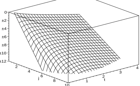
This solution is illustrated in Figure 1. We see that at small times, aggregation is dominant, which rapidly creates an appreciable number of clusters of larger size. At larger times, there is a slower decrease in the concentration of clusters of all sizes. For large cluster sizes (j 1), the maximum concentration occurs at
tc(j)∼
1
Llog
(2L+a%)j
2L
!
. (2.8)
For larger times the solution (2.7), can be approximated by
cj(t)∼
4L2e−Lt a(2L+a%)
a%
2L+a%
!j
, (2.9)
2 4
6 8
10 j
1 2
3 4 t
[image:5.612.77.314.29.175.2]–12 –10 –8 –6 –4 –2 0
Figure 1: Figure of the exact solution (2.7), logcj(t) is plotted against size j and time t, for
1≤j ≤10 and 0< t <4 for the case %= 1, L= 1, a= 1.
From such a solution other quantities of interest may be found, for example the first few moments are given by equation (2.4) and
M1(t) =% e−Lt, M2(t) = %e−Lt
1 + a%
L(1−e −Lt
)
, (2.10)
since
M1(t) = −
∂C
∂z (0, t), M2(t) = ∂2C
∂z2 (0, t). (2.11)
This agrees with the experimental results of Gudmundsson [12] where he observes a decay in the total volume of the material which is exponential. The average cluster size is given by either
M1/M0, or M2/M1, these give similar expressions
M1
M0
= 1 + a% 2L(1−e
−Lt
), M2 M1
= 1 +a%
L(1−e −Lt
). (2.12)
Initially, both give unity, since all material starts in clusters of unit size; as time progresses the former rises steadily to 1 +a%/2L, while the latter approaches 1 +a%/L. A measure of the spread of the distribution can be gained from the polydispersity
M2M0
M2 1
= 1 + a%(1−e
−Lt
) 2L+a%(1−e−Lt
). (2.13)
This quantity is initially equal to one, indicating a monodisperse system and rises to 1+a%/(a%+2L) in the large time limit.
2.2
Size-dependent aggregation rates
In the case ai,j =a(i+j) the coagulation equations have the form
dcj
dt =
1 2a
j−1
X
i=1
jcicj−i−acj ∞
X
i=1
(i+j)ci−Lcj. (2.14)
We use the same generating function as earlier (C(z, t) =
∞
P
j=1cj(t)e
−jz
), to rewrite the above as
∂C ∂t =a
∂C
2 4 6 8 10 j 1 2 3 4 t –12 –10 –8 –6 –4 –2 0
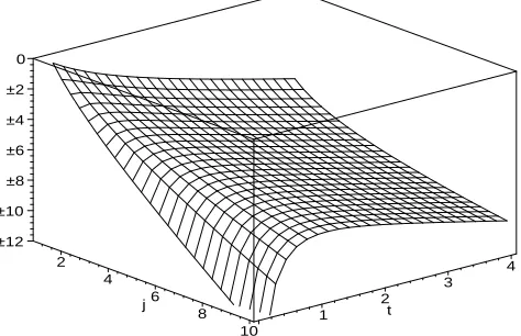
Figure 2: Figure of the exact solution (2.19), logcj(t) is plotted against size j and time t, for
1≤j ≤10 and 0< t <4 for the case %= 1, L= 1, a= 1.
subject to the initial data (2.5), which imply C(z,0) =%e−z
. The mass and number in the system are then governed by
dM1
dt =−LM1,
dM0
dt =−M0(aM1+L), (2.16)
which are solved by
M1(t) = %e
−Lt
, M0(t) =%exp
−Lt− a% L(1−e
−Lt
)
. (2.17)
As with the size-independent kernel, this confirms the exponential decay of the total mass in the system, however this solution is based onλ= 0 and notλ= 2/3, as was assumed by Gudmundsson. The above solutions for M0 and M1 allow solving (2.15) by the method of characteristics, which
gives the implicit solution
−z = logC
% +Lt+ a%
L(1−e −Lt
) + (2.18)
1−exp
−a%
L(1−e −Lt
)
"
1− Ce
Lt
% exp
a%
L(1−e −Lt
)
#
.
This is inverted by use of Lagrange’s expansion (see Abramowitz & Stegun [14], eq 3.6.6), which yields
cj(t) =
%jj−1 j! e
−Lt−T
(1−e−T
)j−1
e−j(1−e−T)
(2.19)
= %e
−Lt jj−1 j! Tb
j−1 e−jTb
(1−Tb),
where T = (%a/L)(1−e−Lt
) andTb = 1−e−T
. This solution is illustrated in Figure 2. The second moment can also be determined, fromdM2/dt= 2aM1M2−LM2, we find
M2(t) =%e
−Lt
exp
2a%
L (1−e −Lt
)
. (2.20)
There are then two ways of defining the typical size of a cluster in the system, which give very similar expressions
M2
M1
= exp
2a%
L (1−e −Lt
)
, M1 M0
= exp
a%
L(1−e −Lt
)
and the polydispersity of the system (which is related to the variance of the cluster size distribution) is given by
M2M0
M2 1
= exp
a%
L(1−e −Lt
)
. (2.22)
All these formulae assume that the initial conditions are monodisperse, that is, given by (2.5).
2.3
The gelling kernel
A natural question to ask is whether the presence of the explicit mass loss term alters gelation. In the absence of a mass loss term (that is if L= 0), the system (1.2) satisfies
djcj
dt =Jj−1−Jj, where Jj =
j
X
k=1
∞
X
n=j+1−k
kan,kcnck. (2.23)
Formally, we have dM1/dt=−limN→∞JN. If this limit is zero then mass is conserved, and if it is
non-zero the system loses mass to a cluster of infinite size, known as the ‘superparticle’ or the ‘gel’. Intuitively we expect that for large enough λ (or L), the shape of the cluster size distribution will be altered at large sizes, and so gelation could be prevented; however for small (possibly negative)
λ or small L, the mass loss term may have no effect on gelation. In the case λ = 0 the system is once again exactly explicitly solvable as we now show. The generating function in this case reduces the differential-difference equation
dcj
dt =
1 2
j−1
X
i=1
ai(j−i)cicj−i−ajcj ∞
X
i=1
ici−Lcj. (2.24)
to
∂C ∂t =
1 2a
∂C ∂z
!2
+aM1
∂C
∂z −LC, (2.25)
with initial data C(z,0) = %e−z
. Definingu=−∂C
∂z we find the partial differential equation
∂u
∂t +a(u−M1(t)) ∂u
∂z =−Lu. (2.26)
2.3.1 Pre-gel behaviour
Equations governing the number and mass of clusters can be found by putting z = 0 into (2.25) and (2.26). This leads to
dM1
dt =−LM1,
dM0
dt =−
1 2M
2
1 −LM0, (2.27)
which have the solutions
M1(t) = %e
−Lt
, M0(t) =%e
−Lt
1− a% 2L(1−e
−Lt
)
. (2.28)
These formulae are only valid in the pre-gelation stage of the process. The partial differential equation (2.26) is solved by the method of characteristics, leading to
z = log%−logu−Lt+ au
L (e
Lt
−1)−a
Z t
In the pregel phase, M1 is given by (2.28) and so we find
e−z
= ue
Lt
% exp − aeLt
L (1−e −Lt
)(u−%e−Lt
)
!
. (2.30)
which can be inverted using Lagrange’s expansion, yielding
cj(t) =
%jj−2 e−Lt j!
%a(1−e−Lt
)
L
!j−1
exp −%aj(1−e
−Lt
)
L
!
, (2.31)
or cj(t) = %e−Ltjj−2Tj−1e−jT/j! where T = %a(1−e−Lt)/L. Note that this new time variable
satisfies T → a%/L as t → ∞. In the limit L → 0 with % = a = 1, this reduces to the classical solution pre-gelation solution, cj(t) = jj−2tj−1e−jt/j!, where gelation occurs att =tg = 1. Thus in
the general solution for L6= 0, gelation occurs at Tg = 1. So if L > %a then gelation is prevented
by the mass loss term since T = 1 is never reached even in the limit t → ∞, whereas for L < %a
gelation is merely delayed from tg = 1/%ato
tg =−
1
Llog 1− L a%
!
. (2.32)
For small Lthis asymptotes to tg ∼(1/%a)(1 +L/2%a); and tg → ∞as L→%a.
In the pre-gel regime the typical cluster size is given by
M1
M0
= 2L
2L−a%(1−e−Lt
),
M2
M1
= Lµ
L%−a%µ(1−e−Lt
), (2.33)
and the polydispersity by
M2M0
M2 1
= 2Lµ−a%µ(1−e
−Lt
)
2L%−2a%µ(1−e−Lt). (2.34)
For general initial data, information on the gelation behaviour of the system can be gained from the second moment. Here we shall not assume that the initial conditions are monodisperse, rather we assume thatM1(0) =%and M2(0) =µ. The second moment is determined bydM2/dt=
aM2
2 −LM2, which shows that for sufficiently large L, the possibility of gelation may be removed.
The solution for M2(t) is
M2(t) =
µL
aµ+ [L−aµ]eLt. (2.35)
The gel-point occurs at the time at which the second moment diverges (that isM2 → ∞ast→tg),
which implies
tg =−
1
Llog 1− L aµ
!
. (2.36)
Thus gelation only occurs if µ > L/a. There is an interesting issue about the sensitive dependence of gelation to initial data: for example, one can perturb the monodisperse initial data (2.5) by adding in a small concentration (of order ε 1) of one particular very large cluster size (size
2.3.2 Post-gel behaviour
As the gel-point is approached (t → tg), a singularity develops, namely uz → −∞ at z = 0; this
corresponds to the divergence in the second moment, M2(t). The post-gel solution is characterised
by persistence of the singularity in uz atz = 0. By differentiating (2.29) with respect to z we find
∂u ∂z =
Lu
au(eLt−1)−L, (2.37)
and so substituting z= 0 into this, we find
M1(t) =u(0, t) =
L
a(eLt−1) for t > tg. (2.38)
It can be checked that at t =tg the formula (2.38) givesM1 =%−L/a as does (2.28), thus M1 is
continuous across the gel-point t=tg.
We now return to (2.29) with M1(t) given by (2.28) for t < tg and by (2.38) fort > tg. In this
latter region we then find
e−z
= eau
L (e
Lt
−1)e−au(eLt−1)/L
, (2.39)
and applying Lagrange’s expansion once again, we obtain
cj(t) =
Ljj−2 e−j
aj!(eLt−1). (2.40)
Thus asj → ∞we have the usual post-gel algebraic decay in cluster size withcj ∼L/
√
2πaj5/2(eLt−
1). Note that: (i) this formula and (2.40) are independent of the initial mass in the system,
%; (ii) (2.40) is a similarity solution of separable form, cj(t) = fj/τ(t); and, (iii) from (2.40)
we determine the number of clusters in the post-gel regime. At t = tg equation (2.28) implies
M0(tg) =%(1−L/a%)/2, which can then be used as initial data for the ordinary differential
equa-tion for M0(t) in (2.27) to yield the post-gel solution
M0(t) =
L
2a(eLt−1), t≥tg. (2.41)
A gelling solution is illustrated in Figure 3, where the gel-time is log 2.
A natural question to consider in this scenario is how much of the initial mass ends up in the gelled form and how much is removed by the explicit mass loss term, and so ends up adhered to the wall. To analyse this, we introduce two new quantities: W(t) is the mass adhered to the wall, and G(t) the mass in the gel. Thus we have M1(t) +G(t) +W(t) = % independent of time. In
the pre-gel phase, G = 0, W = %−M1; and, as t → ∞, M1 → 0, so in the large time limit, we
have G+W = %. We also have dW/dt= P∞
j=1Ljλ+1cj, which, in the case of λ = 0, simplifies to
dW/dt=LM1. In the pre-gel phase of the reaction, integrating dW/dt=LM1 yields
W(t) = (%/L)(1−e−Lt
), (t≤tg), (2.42)
thus at the gel-point we have W(tg) =L/a(assuming monodisperse initial data (2.5)). Integrating
dW/dt=LM1 in the post-gel phase, where M1(t) is given by (2.38), yields
W(t) = L
a 1 + log(1−e −Lt
)−log L
a%
!!
2 4
6 8
10 j
1 2
3 4 t
–12 –10 –8 –6 –4 –2 0
2 4
6 8
10 j
1 2
3 4 t
[image:10.612.59.398.16.177.2]–12 –10 –8 –6 –4 –2 0
Figure 3: The exact solution (2.31) for t < tg and (2.40) for t > tg; logcj(t) is plotted against size
j and time t for 1≤j ≤10 and 0< t <4; on the left for %= 2, L= 1, a = 1, so that the gel-time
tg = log 2; on the right for%= 1, L= 1, a= 1, so that there is no gelation (tg =∞).
0 0.2 0.4 0.6 0.8 1
Phi
0.2 0.4 0.6 0.8 1 1.2 1.4
L/a rho
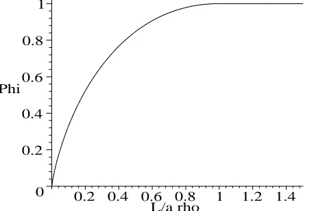
Figure 4: Graph of proportion of mass ultimately adhered to the wall against the dimensionless parameter L/a% which indicates the rate of loss of matter from the system.
Thus, ultimately the mass deposited on the wall and in the gelled form is given by
W∞ = L
a 1−log L a%
!!
, G∞=%−W∞, (2.44)
provided L < a%. If L ≥a% then the mass loss term prevents gelation, and so all mass eventually ends up on the wall. Thus if we look at the proportion of mass adhering to the wall (Φ =W∞/%) as a function of the nondimensional parameter group L/a%we have the function
Φ(L/a%) =
(
(1−log(L/a%))L/a%, L/a% <1,
1, L/a%≥1, (2.45)
which is continuous and has a continuous first derivative, but has a discontinuous second derivative. To illustrate this, we consider values of L/a% close to unity, we put L/a%= 1−ε with 0 < ε 1 and then find that Φ ∼1− 122. Thus Φ rises from zero at L = 0 to its upper limit at L/a% = 1
[image:10.612.82.311.242.396.2]3
Similarity solutions
The existence of similarity solutions to the Smoluchowski coagulation equations has been the subject of much study, analytically, by Kreer & Penrose [15] and da Costa [16] and by asymptotic methods, for example, by Hendriks et al. [17], and more recently by Davies et al. [6]. Gudmundsson [12] speculated on the existence of similarity solutions to the mass-losing coagulation equations. Here we show that such solutions may exist in the case λ <0.
3.1
Size-independent aggregation rates
For ai,j =a, we seek a solution of the formcj(t) =tγf(η) where η =jtβ is the similarity variable.
We substitute the ansatz into equation (1.4), and find that all terms balance, provided β = 1/λ,
γ = 1/λ−1. Since β should be negative, we requireλ also to be negative for a similarity solution of this form to exist. Such a scaling satisfies the density conservation equation dM1/dt=−LMλ+1
since M1 ∼ O(tγ−2β), and Mλ+1 ∼ O(tγ−(λ+2)β). From such calculations we find
M0(t) = Φ0t
−1
, M1(t) = Φ1t
−1−1/λ
, M2(t) = Φ2t
−1−2/λ
, (3.1)
where Φk = R
∞
η=0ηkf(η)dη, and so if M2 is to be well-defined we require λ < −2. The average
cluster size, which is given by M1/M0 or M2/M1, increases according to t−1/λ. The polydispersity
M2M0/M12 is constant (independent of time) once the similarity solution has been approached.
With λ <0, smaller clusters are removed at a faster rate than larger ones, thus the total number of clusters decays faster than the mass in the system, and higher moments diverge more rapidly, leading to a cluster size-distribution in which higher moments cease to exist.
The functionf(η) satisfies
(1−λ)
λ f+ η λ
df dη =
1 2a
Z η
0 f(ξ)f(η−ξ)dξ−aΦ0f −Lη
λf. (3.2)
where Φ0 =
R∞
0 f(ξ)dξ. Unfortunately, in general, such equations are not solvable; however, for
large and small η, asymptotic approximations forf(η) are available.
For smallηthe leading order balance is between the rate of change term,ηf0
(η)/λ, and the mass loss term, Lηλf(η). This gives the expression f(η)
∼ e−Lηλ
. A correction term can be calculated by substituting f(η) =e−Lηλ
g(η) into (3.2). This leads to
1
λ −1
g+ η
λ dg
dη +aΦ0g = 0, (3.3)
at the next order of accuracy, the convolution being much smaller than these terms. This expression is solved by g(η) = Aηq for some amplitude A and exponent q given by q = λ
−1−λaΦ0. Thus
we have the expression
f(η)∼Aηλ−1−λaΦ0
e−Lηλ
, for η1, (3.4)
and
cj(t)∼Ajλ
−1−λaΦ0
t−aΦ0
e−Ljλt
, (3.5)
as t→ ∞ and for j t−1/λ
.
For large η, the leading order balance is between the creation of new clusters as described by the convolution term, the loss by coagulation and the rate of change terms, thus we have
η λ
df dη +
1
λ −1 +aΦ0
f =a
Z η/2
If we assume f(ξ) is given by the small argument asymptotic expansion (3.4) and all the other occurrences of f are given by the large asymptotic expansion f(η) ∼ Bηq for some B, q then we
find that all the terms on the left-hand side of (3.6) balance with the contribution to the integral from the small ξ-range, and that this places no restrictions on the values of B or q. Considering now the part of the integral where ξ∼η, we find that to balance all terms we require q=−1 and then
aΦ0 = 12aB
Z 1 0
dx
x(1−x), (3.7)
where the divergences at the end-points of the integral can be ignored since an alternative expression for f should be used there (3.4). Thus, for large η we have
f(η)∼B/η, as η→+∞, (3.8)
and thus cj ∼B/jt ast→ ∞ with j t−1/λ.
For the coagulation kernel suggested by Gudmundsson, namely ai,j = 2 + (i/j)ω+ (j/i)ω with
ω = 1/3, the scalings for a similarity solution are exactly the same as for the constant kernel
ai,j =a. the equation for the self-similar function f(η) is, however, different, and so has different
large and small η asymptotics.
η λ
df dη +
1
λ −1
f+Lηλf +a2Φ0+ηωΦ−ω+η −ω
Φω
f
= 1 2a
Z η
0 f(ξ)f(η−ξ)
"
2 + η−ξ
ξ
!ω
+ ξ
η−ξ
!ω#
dξ. (3.9)
Hence
f(η)∼Aηqexp −Lηλ+ λaΦω
ωηω
!
as η→0+, (3.10)
for some exponent q and some amplitude A; whilst
f(η)∼Bηω−1
for η1, (3.11)
for some constant B.
3.2
Size-dependent aggregation rates
For ai,j =a(i+j) the coagulation equations have the form
dcj
dt =
1 2a
j−1
X
i=1
jcicj−i−acj ∞
X
i=1
(i+j)ci−Ljλcj. (3.12)
Assuming cj(t) =tγf(j/tβ) we find γ = 2/λ−1, β =−1/λ, and f(η) is determined by
2
λ −1
f +η
λ df dη +Lη
λf(η) +aΦ
1f(η) +aΦ0ηf(η)
= 1 2aη
Z η
0 f(ξ)f(η−ξ)dξ. (3.13)
The regime η=O(1) corresponds to j =O(t−1/λ
), and in general cannot be solved.
In the large time limit, forλ >0, it is the smallηlimit which is of interest, since this corresponds to aggregation sizes j t−1/λ
removed from the system, knowledge of the behaviour of such smaller cluster sizes is more important in physical applications. Thus we consider in more detail the smallηasymptotics solution of (3.13). At leading order the balance is between ηf0
/λand Lηλf which produces the solutionf =e−Lηλ
as in the case of the size-independent coagulation kernel. The first correction term, however differs; we substitute f =e−Lηλ
g(η) to determine the prefactor of the exponent, and obtain the equation
2
λ −1 +aΦ1
g+ η
λ dg
dη = 0, (3.14)
This implies g(η)∼ηλ−2−λaΦ1, and we thus have
f(η)∼Aηλ−2−λaΦ1
e−Lηλ
for η1. (3.15)
The asymptotic solution for cj(t) is then
cj(t) =Ajλ
−2−aλΦ1
t−aΦ1
e−Ljλt
as t→ ∞ with j t−1/λ
. (3.16)
For completeness, we quote the largeηasymptotics; due to the nonlocal nature of (3.13) isolating the large η asymptotics is not straightforward. At large η, the dominant terms are the formation of clusters by the integral term, and the loss by collision with other clusters, thus from (3.13) we aim to solve
aΦ0ηf = 12aη
Z η
0 f(ξ)f(η−ξ)dξ, (3.17)
for whichf(η) =Bηqappears to be a solution forq=
−1 andB = 2Φ0/R01(x(1−x))
−1
dx. However, this integral is divergent. The solution f(η) = Bη−1
remains, since the divergence is caused by integrating the functionf(ξ) near ξ= 0, where f is not given by Bξ−1
but by (3.15) instead. With this modification, the solution f(η) = Bη−1
remains valid for large η, but the expression for B
cannot be evaluated without knowing f(η) across the whole range of values from η= 0 upto large
η. Largeη corresponds to j t−1/λ
and so we have
cj(t)∼
B
jt1−1/λ as t → ∞ with j t −1/λ
. (3.18)
3.3
Gelling kernel
Forai,j =aij we have seen that there is a gelation point if L < aM2(0), and in this case, the
post-gel solution corresponds to a similarity solution; from (2.40) we see that the appropriate scalings are cj(t) = fj/(eLt −1). In the case λ < 0 the loss is predominantly taken from smaller cluster
sizes, with larger cluster sizes having smaller loss rates. Since gelation occurs due to the very slow decay of concentrations with increasing cluster size, loss rates with negative λ will not prevent the formation of a distribution function with a slowly decaying tail. Thus with small L, gelation should still occur, and we expect the post-gel solution to have the form of a similarity solution.
Assuming cj(t) = tγf(jtβ), we find a similarity solution provided β = 1/λ and γ = 3/λ−1.
The form of f(η) is then given by
η λ
df dη +Lη
λf(η) + (3λ
−1)f(η) +aΦ1ηf(η)
= 12a
Z η
A solution of this equation is not available explicitly, however, some properties of the solution can be deduced by considering the small and large η behaviour of a solution. Also the behaviour of certain quantities can be derived, for example
M0(t)∼t2/λ
−1
Z ∞
0 f(η)dη, M1(t)∼t 1/λ−1
Z ∞
0 ηf(η)dη. (3.20)
For small η, the leading order balance is between the rate of change term ηf0
(η)/λ and the loss term Lηλf(η) leading to f(η) = g(η)e−Lηλ
as in previous cases. The correction term is then determined by solving
3
λ −1
g +η
λ dg
dη = 0, (3.21)
the convolution term being smaller than these retained terms. From the above equation we find
g(η) =Aηλ−3
thus we have
cj(t)∼Ajλ
−3 e−Ljλt
as t→ ∞ for j t−1/λ
, (3.22)
for some constant A.
For large η, the leading order balance is
aΦ1ηf = 12a
Z η
0 ξf(ξ)(η−ξ)f(η−ξ)dξ, (3.23)
that is, between for the formation of clusters of scaled size η by coagulation and the loss by coagulation. This leads to the asymptotic expression f(η)∼B/η2 for some constant B. Thus, we
have
cj(t)∼
B
j2t1−1/λ as t→ ∞ with j t −1/λ
. (3.24)
3.4
More general coagulation kernels
We consider some more general coagulation kernels, and show that the above analysis remains applicable. For the general coagulation kernel ai,j =a(ij)α(iβ+jβ) we find the similarity variable
is η = jt1/λ again, with the concentrations c
j(t) being given by t−1+(1+2α+β)/λf(η). The function
f(η) is then given by
η λ
df
dη − 1−
1 + 2α+β λ
!
f+Lηλf +a(Φα+β +ηβΦα)ηαf
= 1 2a
Z η ξ=0ξ
αf(ξ)(η
−ξ)αf(η−ξ)(ξβ+ (η−ξ)β)dξ (3.25)
Assumingα, β >0 we find the following asymptotic results hold: forη1,f(η)∼ηλ−1−2α−β e−Lηλ
, thus
cj(t)∼Ajλ
−1−2α−β e−Ljλt
, as t→ ∞ with j t−1/λ
; (3.26)
and f(η)∼Bη−1−α
when η1, thus
cj(t)∼Bj1/λt
−1+(α+β)/λ
as t→ ∞ with j t−1/λ
. (3.27)
eta1e-3 1e-2 1e-4
1e-5 1
0.8
0.6
0.4
0.2
[image:15.612.105.346.20.163.2]0
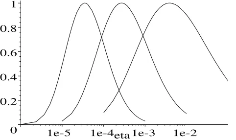
Figure 5: Graph of the similarity function f(η)/f(ηc) against logη for small η; for the kernels
ai,j = 1 (on the right), ai,j =i+j (in the centre), ai,j =ij (on the left).
we obtain the similarity solution cj ∼ t(1−λ−β)/λf(η) with η = jt1/λ. For small η the asymptotic
solution is f(η)∼Aηqexp(−Lηλ+λaΦ
0η−β/β) with q=β+λ−1−λaΦ−β, implying
cj(t) ∼ Ajqt1/λ
−aΦ
−βexp−Ljλt+ λaΦ0
βjβtβ/λ
!
as t→∞ with jt−1/λ .
(3.28)
However, in the application we are concerned with here, which is a stirred chamber, the case of aggregation in a linear shear velocity profile is perhaps more relevant. This corresponds to
ai,j = (i1/3 +j1/3)3, and so following analysis similar to the above, we find the similarity solution
cj(t) = t−1+2/λf(jt1/λ), where the distribution f(η) is given by f(η) ∼ Aηpe−Lη
λ
as t → ∞ for
j t−1/λ
; here the constants A, pmust satisfyp=λ−2−λaΦ1 whereλ <0 and Φ1 =R
∞
0 ξf(ξ)dξ.
3.5
Small
η
results
For each of the kernels considered above, the small η asymptotics have the form f(η) =Aηqe−Lηλ
with q < 0. This has the form of a single-humped function, with maximum at ηc = (q/λL)1/λ.
Thus provided this occurs atηc1, the form of the similarity solution will also be single-humped,
the maximum having amplitude f(ηc) = Aqe−q/λ/λL. The form of such functions is illustrated in
Figure 5, where results are shown for the case L= 1, a= 1, Φ0 = 1, Φ1 = 1.2,λ=−0.25.
4
Match to experimental results
The exact solutions given in Section 2 did not have the form observed in the numerical simulations of Gudmundsson (see Gudmundsson [12] and Gudmundsson et al. [18]). One reason for this may be the differences in the kernel used; in numerical work, Gudmundsson used the more accurate kernel ai,j = 2 + (i/j)1/3 + (j/i)1/3 for Brownian coagulation, whereas the theory of Section 2
considered the simpler kernels ai,j =a, ai,j =a(i+j). Another reason is that in Section 2 we only
form of initial data, for example, a single-humped size distribution as given by
cj(0) =Aje
−jξ
, (4.1)
for some ξ. The maximum of this distribution occurs at j = 1/ξ. Using such initial data, with the exact method of solution outlined in Section 2 can still be applied, although the algebra is more complicated.
The initial data for the system are
C(z,0) = A e
z+ξ
(ez+ξ−1)2, M0(0) =
Aeξ
(eξ−1)2, (4.2)
where M0 is the number of clusters, and the mass M1 is initially given by M1(0) = −Cz(0,0) =
Aeξ(eξ+ 1)/(eξ
−1)3. Solving (2.3) for the number of clusters we find
M0(t) =
2LM0(0)
(2L+aM0(0))eLt−aM0(0)
. (4.3)
The kinetic equation (2.2) can then be solved, by using the transformationw= 1/C which linearises the problem and so can be solved by standard methods, which yield
C(z, t) = α
β(ez+ξ−2 +e−z−ξ)
−γ, (4.4)
where
α = 4AL
2(aM
0(0) + 2L)eLt
[aM0(0)(eLt−1) + 2LeLt]
(4.5)
β = (aM0(0) + 2L)[aM0(0)(eLt−1) + 2LeLt] (4.6)
γ = aA(eLt−1)(aM0(0) + 2L). (4.7)
From this we obtain the explicit solution
ck(t) =
α β
(k−1)/2
X
j=0
k−j−1
j
!
(−1)j 2 + γ
β
!m−2j−1 e−kξ
, k odd,
α β
(k−2)/2
X
j=0
k−j−1
j
!
(−1)j 2 + γ
β
!m−2j−1 e−kξ
, k even.
(4.8)
To assess how the width of the distribution varies in time, we calculate the standard deviation of the distribution σ =√((M2M0−M12)/M12). This is determined by
σ2 = 12sech2(12ξ)
"
1 + aA(e
Lt
−1) coshξ aA(eLt−1) + 8LeLtsinh2 1
2ξ
#
. (4.9)
j 30 40 50 20
10 2
1.5
1
0.5
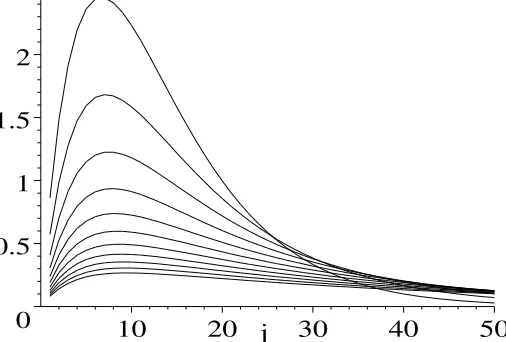
[image:17.612.93.346.20.191.2]0
Figure 6: Plots of the distribution (4.8) in the case L = 1, a = 1, ξ = 0.15, A = 1. The concentration ck(t) is plotted against aggregation size k for times fromt= 0 to t = 0.1 in steps of
size t = 0.01.
5
Conclusions
We have considered a variety of aggregation kernels which permit exact explicit solutions to be derived in the pure aggregation case. To these coagulation equations we have added a general mass loss term. In the case of size-independent mass loss rates, explicit solutions are still available, and we have derived these in Section 2. Due to the presence of stirring in the system under consideration here, fractal clusters observed in Diffusion-Limitted Aggregation (DLA) do not play an important role in the kinetics of growth analysed here, instead more compact aggregates are found [12].
The most interesting of these cases is the kernel ai,j =aij, for which gelation is known to exist
in the mass-conserving case. With a mass loss term present, we find that the existence of a gelation transition depends on the strength of the mass loss term. For small mass loss terms, the gelation phenomenon persists, albeit with the gelation time delayed due to the presence of the mass loss term. For stronger mass loss terms, gelation is completely removed from the system. Our analysis precisely determines how strong the mass loss term should be to prevent gelation.
When the mass loss term is allowed to be size-dependent, explicit solutions are no longer avail-able, and instead, we have sought similarity solutions. These have been found in the cases where mass loss decreases with increasing size, in particular, in Section 3.4 we examined the case of a loss term of the form L(cj) = Ljλcj with λ < 0, for which similarity solutions have the form
cj(t) =t−1+(1+2α+β)/λf(jt1/λ), where the aggregation kernel is ai,j =a(ij)α(iβ+jβ).
The explicitly solvable case, λ = 0, shows no self-similar behaviour and so we postulate that in the case λ > 0, similarity solutions also fail to exist. However, in the case λ = 0, and ai,j = a
References
[1] TA Engh. Principles of Metal Refining. Oxford University Press, Oxford, (1992).
[2] CJ Simensen. The effect of melt refining upon inclusions in aluminum. Metall. Trans. B,13B, 31–34, (1982).
[3] DG McCartney. Grain refining of aluminium and its alloys. Int. Mater. Rev., 34, 247–260, (1989).
[4] JP Martin, F Painchaud. On-line metal cleanliness determination in molten aluminium alloys using the LiMCA II analyser. In ‘Light Metals’, ed. V Mannweiler, The Minerals, Metals and Materials Society, Warrendale, PA, 915–920, (1994).
[5] F Leyvraz & HR Tschudi. Singularities in the kinetics of coagulation processes. J Phys A:
Math Gen,14, 3389–3405, (1981).
[6] SC Davies, JR King & JAD Wattis. Self-similar behaviour in the coagulation equations.J Eng Math, 36, 57–88, (1999).
[7] SC Davies, JR King & JAD Wattis. The Smoluchowski coagulation equations with continuous injection. J. Phys A; Math Gen, 32, 7745–7763, (1999).
[8] JAD Wattis, SC Davies & JR King. The Smoluchowski coagulation equations with cluster-gel interactions. preprint, (2003).
[9] P Singh & GJ Rodgers. Coagulation processes with mass loss. J. Phys. A. Math Gen, 29, 437–450, (1996).
[10] EM Hendriks. Exact solution of coagulation equation with removal term.J Phys A: Math Gen,
17, 2299–2303, (1984).
[11] HC Rotstein, A Novick-Cohen & R Tannenbaum. Gelation and cluster growth with cluster-wall interactions. J Stat Phys, 90, 119–143, (1998).
[12] T Gudmundsson. Agglomeration of TiB2 particles in liquid aluminium. PhD thesis,
Notting-ham, (1996).
[13] FP da Costa. A finite dimensional dynamical model for gelation in coagulation processes. J Nonlinear Sci, 8, 619–653, (1998).
[14] M Abramowitz & IA Stegun. Handbook of Mathematical Functions. Dover, New York, (1972)
[15] M Kreer & O Penrose. Proof of dynamic scaling in Smoluchowski’s coagulation equation with constant kernels. J Stat Phys, 74, 389–407, (1994).
[16] FP da Costa. On the dynamic scaling behaviour of solutions to the discrete Smoluchowski equations. Proc Edinburgh Math Soc,39, 547–559, (1996).
[17] EM Hendriks, MH Ernst & RM Ziff. Coagulation equations with gelation. J Stat Phys, 31, 519–563, (1983).