Permutation inference for the general linear model

(1)

http://wrap.warwick.ac.uk/

Original citation:

Winkler, Anderson M., Ridgway, Gerard R., Webster, Matthew A., Smith, Stephen M.

and Nichols, Thomas E.. (2014) Permutation inference for the general linear model.

NeuroImage, Volume 2 . pp. 381-397.

Permanent WRAP url:

http://wrap.warwick.ac.uk/65670

Copyright and reuse:

The Warwick Research Archive Portal (WRAP) makes this work of researchers of the

University of Warwick available open access under the following conditions.

This article is made available under the Creative Commons Attribution- 3.0 Unported

(CC BY 3.0) license and may be reused according to the conditions of the license. For

more details see

http://creativecommons.org/licenses/by/3.0/

A note on versions:

The version presented in WRAP is the published version, or, version of record, and may

be cited as it appears here.

(2)

Permutation inference for the general linear model

Anderson M. Winkler

a,b,c,

⁎

_{, Gerard R. Ridgway}

d

_{, Matthew A. Webster}

a

_,

Stephen M. Smith

a

, Thomas E. Nichols

a,e

a

Oxford Centre for Functional MRI of the Brain, University of Oxford, Oxford, UK b

Global Imaging Unit, GlaxoSmithKline, London, UK c

Department of Psychiatry, Yale University School of Medicine, New Haven, CT, USA d

Wellcome Trust Centre for Neuroimaging, UCL Institute of Neurology, London, UK e

Department of Statistics & Warwick Manufacturing Group, University of Warwick, Coventry, UK

a b s t r a c t

a r t i c l e i n f o

Article history:

Accepted 31 January 2014 Available online 11 February 2014

Keywords:

Permutation inference Multiple regression General linear model Randomise

Permutation methods can provide exact control of false positives and allow the use of non-standard statistics, making only weak assumptions about the data. With the availability of fast and inexpensive computing, their main limitation would be some lack ofﬂexibility to work with arbitrary experimental designs. In this paper we report on results on approximate permutation methods that are moreﬂexible with respect to the experimental design and nuisance variables, and conduct detailed simulations to identify the best method for settings that are typical for imaging research scenarios. We present a generic framework for permutation inference for complex general linear models (GLMs) when the errors are exchangeable and/or have a symmetric distribution, and show that, even in the presence of nuisance effects, these permutation inferences are powerful while providing excellent control of false positives in a wide range of common and relevant imaging research scenarios. We also demonstrate how the inference onGLMparameters, originally intended for independent data, can be used in certain special but useful cases in which independence is violated. Detailed examples of common neuroimaging applications are provided, as well as a complete algorithm–the“randomise”algorithm–for permutation infer-ence with theGLM.

Introduction

Theﬁeld of neuroimaging has continuously expanded to encompass an ever growing variety of experimental methods, each of them produc-ing images that have different physical and biological properties, as well as different information content. Despite the variety, most of the strate-gies for statistical analysis can be formulated as a general linear model (GLM) (Christensen, 2002; Scheffé, 1959; Searle, 1971). The common strategy is to construct a plausible explanatory model for the observed data, estimate the parameters of this model, and compute a suitable statistic for hypothesis testing on some or all of these parameters. The rejection or acceptance of a hypothesis depends on the probability of

ﬁnding, due to chance alone, a statistic at least as extreme as the one observed. If the distribution of the statistic under the null hypothesis is known, such probability can be ascertained directly. In order to be valid, theseparametric testsrely on a number of assumptions under which such distribution arises and can be recovered asymptotically.

Strategies that may be used when these assumptions are not guaran-teed to be met include the use ofnon-parametric tests.

Permutation testsare a class of non-parametric methods. They were pioneered byFisher (1935a)andPitman (1937a,b, 1938). Fisher dem-onstrated that the null hypothesis could be tested simply by observing, after permuting observations, how often the difference between means would exceed the difference found without permutation, and that for such test, no normality would be required. Pitman provided theﬁrst complete mathematical framework for permutation methods, although similar ideas, based on actually repeating an experiment many times with the experimental conditions being permuted, can be found even earlier (Peirce and Jastrow, 1884). Important theoretical and practical advances have been ongoing in the past decades (Edgington, 1995; Good, 2002, 2005; Kempthorne, 1955; Lehmann and Stein, 1949; Pearson, 1937; Pesarin and Salmaso, 2010; Scheffé, 1943; Westfall and Troendle, 2008), and usage only became practical after the availability sufﬁcient computing power (Efron, 1979).

In neuroimaging, permutation methods wereﬁrst proposed byBlair et al. (1994)for electroencephalography, and later byHolmes et al. (1996)for positron-emission tomography, with the objective of allowing inferences while taking into account the multiplicity of tests. These early permutation approaches already accounted for the spatial smoothness of the image data.Arndt et al. (1996)proposed a permutation scheme for ⁎ Corresponding author at: Oxford Centre for Functional MRI of the Brain, University of

Oxford, Oxford, UK.

E-mail address:winkler@fmrib.ox.ac.uk(A.M. Winkler). URL:http://www.fmrib.ox.ac.uk(A.M. Winkler).

http://dx.doi.org/10.1016/j.neuroimage.2014.01.060

NeuroImage

(3)

testing the omnibus hypothesis of whether two sets of images would dif-fer. Structural magnetic resonance imaging (MRI) data were considered by

Bullmore et al. (1999), who developed methods for omnibus, voxel and cluster-mass inference, controlling the expected number of false positives.

Single subject experiments from functional magnetic resonance im-aging (FMRI) presents a challenge to permutation methods, as serial au-tocorrelation in the time series violates the fundamental assumption needed for permutation, that of exchangeability (discussed below). Even though some early work did not fully account for autocorrelation (Belmonte and Yurgelun-Todd, 2001), other methods that accommo-dated the temporally correlated nature of theFMRIsignal and noise were developed (Brammer et al., 1997; Breakspear et al., 2004; Bullmore et al., 1996, 2001; Laird et al., 2004; Locascio et al., 1997). Some of these methods use a single reference distribution constructed by pooling permutation statistics over space from a small number of random permutations, under the (untenable and often invalid) assump-tion of spatial homogeneity of distribuassump-tions.

Nichols and Holmes (2002)provided a practical description of permutation methods forPETand multi-subjectFMRIstudies, but noted the challenges posed by nuisance variables. Permutation inference is grounded onexchangeabilityunder the null hypothesis, that data can be permuted (exchanged) without affecting its joint distribution. How-ever, if a nuisance effect is present in the model, the data cannot be con-sidered exchangeable even under the null hypothesis. For example, if one wanted to test for sex differences while controlling for the linear ef-fect of age, the null hypothesis is“male mean equals female mean”, while allowing age differences; the problem is that, even when there is no sex effect, a possible age effect may be present, e.g., younger and older individuals being different, then the data are not directly ex-changeable under this null hypothesis. Another case where this arises is in factorial experiments, where one factor is to be tested in the pres-ence of another, or where their interaction is to be tested in the prespres-ence of main effects of either or both. Although permutation strategies for factorial experiments in neuroimaging were considered bySuckling and Bullmore (2004), a more complete general framework to account for nuisance variables is still missing.

In this paper we review the statistical literature for theGLMwith arbi-trary designs and contrasts, emphasising useful aspects, yet that have not been considered for neuroimaging, unify this diverse set of results into a single permutation strategy and a single generalised statistic, pres-ent implempres-entation strategies for efﬁcient computation and provide a complete algorithm, conduct detailed simulations and evaluations in various settings, and identify certain methods that generally outper-forms others. We will not consider intrasubject (timeseries)FMRIdata, fo-cusing instead on modelling data with independent observations or sets of non-independent observations from independent subjects. We give examples of applications to common designs and discuss how these methods, originally intended for independent data, can in special cases be extended, e.g., to repeated measurements and longitudinal designs.

Theory

Model and notation

At each spatial point (voxel, vertex or face) of an image representa-tion of the brain, a general linear model (Searle, 1971) can be formulat-ed and expressformulat-ed as:

Y¼Mψþϵ ð1Þ

whereYis theN× 1 vector of observed data,1_M_{is the full-rank}_N_{× r}

design matrix that includes all effects of interest as well as all modelled

nuisance effects,ψis ther× 1 vector ofrregression coefﬁcients, andϵis theN× 1 vector of random errors. In permutation tests, the errors are not assumed to follow a normal distribution, although some distri-butional assumptions are needed, as detailed below. Estimates for the regression coefﬁcients can be computed asψ^¼MþY, where the super-script (+_{) denotes the Moore}

–Penrose pseudo-inverse. Our interest is to test the null hypothesis that an arbitrary combination (contrast) of some or all of these parameters is equal to zero, i.e.,H0:C′ψ= 0, whereCis ar×sfull-rank matrix ofscontrasts, 1≤s≤r.

For the discussion that follows, it is useful to consider a transforma-tion of the model in Eq.(1)into a partitioned one:

Y¼XβþZγþϵ ð2Þ

whereXis the matrix with regressors of interest,Zis the matrix with nui-sance regressors, andβandγare the vectors of regression coefﬁcients. Even though such partitioning is not unique, it can be deﬁned in terms of the contrastCin a way that inference onβis equivalent to inference onC′ψ, as described inAppendix A. As the partitioning depends onC, if more than one contrast is tested,XandZchange for each of them.

As the models expressed in Eqs.(1) and (2)are equivalent, their re-siduals are the same and can be obtained as^ϵ¼RMY, whereRM=I− HMis the residual-forming matrix,HM=MM+_{is the projection (}_“_hat_”₎ matrix, andIis theN×Nidentity matrix. The residuals due to the nuisance alone are^ϵZ¼RZY, whereRZ=I−HZ, andHZ=ZZ+. For

per-mutation methods, an important detail of the linear model is the non-independence of residuals, even when errors_ϵare independent and have constant variance, a fact that contributes to render these methods approximately exact. For example, in that setting E Varð ð^ϵZÞÞ ¼RZ≠I.

The commonly usedFstatistic can be computed as (Christensen, 2002):

F¼ ^

ψ′C C′M′M−1C

−1

C′^ψ

rankð ÞC = ^ϵ ′_^_ϵ

N−rankð ÞM

¼β^ ′

X′X

^ β

rank_{ð Þ}C = ^

ϵ′^ϵ

N₋rank_{ð Þ−}X rank_{ð Þ}Z :

ð3Þ

When rankð Þ ¼C 1;βîs a scalar and the Student'ststatistic can be expressed as a function ofFast¼sign ffiffiffiffiβ^ pF.

Choice of the statistic

In non-parametric settings we are not constrained to theFort statis-tics and, in principle, any statistic where large values reﬂect evidence against the null hypothesis could be used. This includes regression

coef-ficients or descriptive statistics, such as differences between medians, trimmed means or ranks of observations (Ernst, 2004). However, the statistic should be chosen such that it does not depend on the scale of measurement or on any unknown parameter. The regression coeffi -cients, for instance, whose variance depends both on the error variance and on the collinearity of that regressor with the others, are not in prac-tice a good choice, as certain permutation schemes alter the collinearity among regressors (Kennedy and Cade, 1996). Specifically with respect to brain imaging, the correction for multiple testing (discussed later) re-quires that the statistic has a distribution that is spatially homogeneous, something that regression coefficients cannot provide. In parametric settings, statistics that are independent of any unknown parameters are calledpivotal statistics. Statistics that are pivotal or asymptotically pivotal are appropriate and facilitate the equivalence of the tests across the brain, and their advantages are well established for related non-parametric methods (Hall and Wilson, 1991; Westfall and Young, 1993). Examples of such pivotal statistics include the Student'st, theF

ratio, the Pearson's correlation coefﬁcient (often known asr), the

coef-ﬁcient of determination (R2), as well as most other statistics used to construct conﬁdence intervals and to compute p-values in parametric tests. We will return to the matter of pivotality when discussing 1

(4)

exchangeability blocks, and the choice of an appropriate statistic for these cases.

p-Values

Regardless of the choice of the test statistic, p-values offer a common measure of evidence against the null hypothesis. For a certain test statis-ticT, which can be any of those discussed above, and a particular ob-served value T0 of this statistic after the experiment has been conducted, the p-value is the probability of observing, by chance, a test statistic equal or larger than the one computed with the observed values, i.e.,P(T≥T0|H0). Although here we only consider one-sided tests, where evidence againstH0corresponds to larger values ofT0, two-sided or negative-valued tests and their p-values can be similarly defined. In parametric settings, under a number of assumptions, the p-values can be obtained by referring to the theoretical distribution of the chosen statistic (such as theFdistribution), either through a known formula, or using tabulated values. In non-parametric settings, these assumptions are avoided. Instead, the data are randomly shuffled, many times, in a manner consistent with the null hypothesis. The model isfitted repeatedly once for every shuffle, and for eachfit a new realisa-tion of the statistic,Tj⁎, is computed, beingja permutation index. An

em-pirical distribution ofT⁎under the null hypothesis is constructed, and

from this null distribution a p-value is computed as1

J∑jI T⁎j≥T0

, whereJis the number of shufﬂings performed, andI(∙) is the indicator function. From this it can be seen that the non-parametric p-values are discrete, with each possible p-value being a multiple of 1/J. It is im-portant to note that the permutation distribution should include the ob-served statistic without permutation (Edgington, 1969; Phipson and Smyth, 2010), and thus the smallest possible p-value is 1/J, not zero.

Permutations and exchangeability

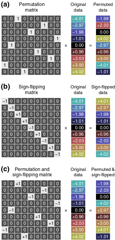
Perhaps the most important aspect of permutation tests is the man-ner in which data are shufﬂed under the null hypothesis. It is the null hypothesis, together with assumptions about exchangeability, which determines the permutation strategy. Let thej-th permutation be expressed byPj, aN×Npermutation matrix, a matrix that has all

ele-ments being either 0 or 1, each row and column having exactly one 1 (Fig. 1a). Pre-multiplication of a matrix byPjpermutes its rows. We

de-noteP ¼ Pj the set of all permutation matrices under consideration, indexed by the subscriptj. We similarly deﬁne a signﬂipping matrixSj,

aN×Ndiagonal matrix whose non-zero elements consist only of +1 or−1 (Fig. 1b). Pre-multiplication of a matrix bySjimplements a set

of signﬂips for each row. Likewise,S ¼ Sj denotes the set of all sign

ﬂipping matrices under consideration. We consider also both schemes together, whereBj¼Pj′Sj″implements signﬂips followed by permuta-tion; the set of all possible such transformations is denoted asB= {Bj}.

Throughout the paper, we use generic terms asshufflingor rearrange-mentwhenever the distinction between permutation, signflipping or combined permutation with signflipping is not pertinent. Finally, letβ^j andTj⁎, respectively, be the estimated regression coefficients

and the computed statistic for the shufﬂingj.

The essential assumption of permutation methods is that, for a given set of variables,their joint probability distribution does not change if they are rearranged. This can be expressed in terms of exchangeable errors or independent and symmetric errors, each of these weakening different assumptions when compared to parametric methods.

Exchangeable errors(EE) is the traditional permutation requirement (Good, 2005). The formal statement is that, for any permutationPj∈P, ϵd

Pjϵ, where the symbold denotes equality of distributions. In other words, the errors are considered exchangeable if their joint distribution is invariant with respect to permutation. Exchangeability is similar to, yet more general than, independence, as exchangeable errors can have all-equal and homogeneous dependence. Relative to the common

parametric assumptions of independent, normally and identically dis-tributed (iid) errors,EErelaxes two aspects. First, normality is no longer assumed, although identical distributions are required. Second, the independence assumption is weakened slightly to allow exchangeability when the observations are not independent, but their joint distribution is maintained after permutation. While exchangeability is a general con-dition that applies to any distribution, we note that the multivariate normal distribution is indeed exchangeable if all off-diagonal elements of the covariance matrix are identical to each other (not necessarily equal to zero) and all the diagonal elements are also identical to each other. In parametric settings, such dependence structure is often re-ferred to ascompound symmetry.

Independent and symmetric errors (ISE) can be considered for measurements that arise, for instance, from differences between two groups if the variances are not assumed to be the same. The formal statement for permutation underISEis that for any signﬂipping matrix Sj∈S;ϵdSjϵ, that is, the joint distribution of the error terms is invariant with respect to signﬂipping. Relative to the parametric assumptions of independent, normally and identically distributed errors,ISErelaxes normality, although symmetry (i.e., non-skewness) of distributions is

−4.01 −2.97 −1.98 0.00 +0.96 −1.01 +3.00 +4.02 +2.03 Permutation matrix Original data Permuted data

0 0 0 0 0

0 0 0 0

0 0 0

0 0 0 0

0 0 0

0 0 0 0 0 0 0 0 0

0 0 0

1

0 0 0

0 0 0 0 0

0 0

0 0 0 0

0 0

0 0 0 0 0 0 0 0 0 0 0 0 0 0 0 0 1 1 1 1 1 1 1 1 −4.01 −2.97 −1.98 0.00 +0.96 −1.01 +3.00 +4.02 +2.03

(a)

+4.01 +2.97 −1.98 0.00 +0.96 −1.01 +3.00 −4.02 −2.03 −4.01 −2.97 −1.98 0.00 +0.96 −1.01 +3.00 +4.02 +2.03 Sign-flipping matrix Original data Sign-flipped data

0 0 0 0

0 0 0

0 0 0 0

0 0 0

0 0 0 0 0 0 0 0 0 0 0 0

0 0 0

0 0 0 0 0 0 0 0 0 0 0 0 0

0 0 0 0 0 0 0 0 0 0 0 0 0 0 0 0 0 0 0 0 0 0 −1 −1 +1 +1 −1 +1 0 −1 −1 +1

(b)

+4.01 +2.97 −1.98 0.00 +0.96 −1.01 +3.00 −4.02 −2.03 × = × = × = Permutation and sign-flipping matrix Original data Permuted & sign-flipped

0 0 0 0 0

0 0 0 0

0 0 0

0 0 0 0

0 0 0

0 0 0 0 0 0 0 0 0 0 0 0

+1

0 0

0 0 0 0

0

0 0 0 0 0 0 0

0 0 0 0 0 0

0 0 0 0 0

[image:4.595.338.532.53.456.2]

0 0 0 0 0 0 0 0 0 0 0 0 0 −1 −1 −1 −1 +1 +1 −1 +1 −4.01 −2.97 −1.98 0.00 +0.96 −1.01 +3.00 +4.02 +2.03

(c)

(5)

required. Independence is also required to allow signﬂipping of one observation without perturbing others.

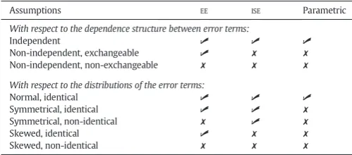
The choice betweenEEandISEdepends on the knowledge of, or as-sumptions about, the error terms. Although theEEdoes not require sym-metry for the distribution of the error terms, it requires that the variances and covariances of the error terms are all equal, or have a structure that is compatible with the definition of exchangeability blocks (discussed below). While theISEassumption has yet more strin-gent requirements, if bothEEandISEare plausible and available for a given model, permutations and signflippings can be performed togeth-er, increasing the number of possible rearrangements, a feature particu-larly useful for studies with small sample sizes. The formal statement for shuffling under bothEEandISEis that, as with the previous cases, for any matrixBj∈β;ϵdBjϵ, that is, the joint distribution of the error terms re-mains unchanged under both permutation and signflipping. A summa-ry of the properties discussed thus far and some bene_fits of permutation methods are shown inTable 1.

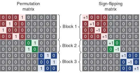
There are yet other important aspects related to exchangeability. The experimental design may dictate blocks of observations that are jointly exchangeable, allowing data to be permuted within block or, alterna-tively, that the blocks may themselves be exchangeable as a whole. This is the case, for instance, for designs that involve multiple observa-tions from each subject. While permutation methods generally do not easily deal with non-independent data, the deﬁnition of these exchange-ability blocks(EB) allows these special cases of well structured depen-dence to be accommodated. Even though the EBs determine how the data shufﬂings are performed, they should not be confused with

variance groups(VG), i.e., groups of observations that are known or assumed to have similar variances, which can be pooled for estimation and computation of the statistic. Variance groups need to be compatible with, yet not necessarily identical to, the exchangeability blocks, as discussed inRestricted exchangeability.

Unrestricted exchangeability

In the absence of nuisance variables, the model reduces toY=Xβ+ϵ, and under the null hypothesisH0:β= 0, the data are pure error,Y=ϵ. Thus theEEorISEassumptions on theerror(presented above) justify freely permuting or signﬂipping thedataunderH0. It is equivalent, however, to alter the design instead of the data. For example, for a nuisance-free design,

PY_¼X_β_þ_ϵ_⇔Y_¼P′X_β_þP′_ϵ _ð4_Þ

since permutation matricesPare orthogonal; the same holds for sign

ﬂipping matricesS. This is an important computational consideration as altering the design is much less burdensome than altering the

image data. The errorsϵare not observed and thus never directly al-tered; going forward we will suppress any notation indicating permuta-tion or sign_ﬂipping of the errors.

In the presence of nuisance variables (Eq.2), however, the problem is more complex. If the nuisance coefﬁcientsγwere somehow known, an exact permutation test would be available:

Y−Zγ¼PXβþϵ: ð5Þ

The perfectly adjusted dataY−Zγare then pure error underH0 and inference could proceed as above. In practice, the nuisance coefﬁ -cients have to be estimated and the adjusted data will not behave asϵ. An obvious solution would be to use the nuisance-only residuals^ϵZas

the adjusted data. However, as noted above, residuals induce dependence and anyEEorISEassumptions onϵwill not be conveyed to

^ϵZ.

A number of approaches have been proposed to produce approxi-mate p-values in these cases (Beaton, 1978; Brown and Maritz, 1982; Draper and Stoneman, 1966; Edgington, 1995; Freedman and Lane, 1983; Gail et al., 1988; Huh and Jhun, 2001; Jung et al., 2006; Kennedy, 1995; Kherad-Pajouh and Renaud, 2010; Levin and Robbins, 1983; Manly, 2007; Oja, 1987; Still and White, 1981; ter Braak, 1992; Welch, 1990). We present these methods in a common notation with detailed annotation inTable 2. While a number of authors have made

comparisons between some of these methods (Anderson and

[image:5.595.301.551.410.503.2]

Legendre, 1999; Anderson and Robinson, 2001; Anderson and ter Braak, 2003; Dekker et al., 2007; Gonzalez and Manly, 1998; Kennedy, 1995; Kennedy and Cade, 1996; Nichols et al., 2008; O'Gorman, 2005;

Table 1

Compared with parametric methods, permutation tests relax a number of assumptions and can be used in a wider variety of situations. Some of these assumptions can be further relaxed with the deﬁnition of exchangeability blocks.

Assumptions EE ISE Parametric

With respect to the dependence structure between error terms:

Independent ✓ ✓ ✓

Non-independent, exchangeable ✓ ✗ ✗

Non-independent, non-exchangeable ✗ ✗ ✗

With respect to the distributions of the error terms:

Normal, identical ✓ ✓ ✓

Symmetrical, identical ✓ ✓ ✗

Symmetrical, non-identical ✗ ✓ ✗

Skewed, identical ✓ ✗ ✗

Skewed, non-identical ✗ ✗ ✗

✓Can be used directly if the assumptions regarding dependence structure and distribution of the error terms are both met.

[image:5.595.33.283.608.718.2]

✗Cannot be used directly, or can be used in particular cases.

Table 2

A number of methods are available to obtain parameter estimates and construct a reference distribution in the presence of nuisance variables.

Method Model

Draper–Stonemana _Y₌_PX_β₊_Z_γ₊_ϵ

Still–Whiteb _PRZY₌_X_β₊_ϵ

Freedman–Lanec

(PRZ+HZ)Y=Xβ+Zγ+ϵ

Manlyd

PY=Xβ+Zγ+ϵ

ter Braake

(PRM+HM)Y=Xβ+Zγ+ϵ

Kennedyf

PRZY=RZXβ+ϵ

Huh–Jhung _PQ_′_RZY₌_Q_′_RZX_β₊_ϵ

Smithh _Y₌_PRZX_β₊_Z_γ₊_ϵ

Parametrici

Y=Xβ+Zγ+ϵ,ϵ∼N(0,σ2 I) a

Draper and Stoneman (1966). This method was called“Shufﬂe Z”by (Kennedy, 1995), and using the same notation adopted here, it would be called“Shufﬂe X”.

b _{Gail et al. (1988); Levin and Robbins (1983); Still and White (1981)}_{. Still and White} considered the specialANOVAcase in whichZare the main effects andXthe interaction.

c

Freedman and Lane (1983). d

Manly (1986); Manly (2007). e

ter Braak (1992). The null distribution for this method considersβ^j¼β^, i.e., the permutation happens under the alternative hypothesis, rather than the null.

f

Kennedy (1995); Kennedy and Cade (1996). This method was referred to as “Residualize both Y and Z”in the original publication, and using the same notation adopted here, it would be called“Residualize both Y and X”.

g

Huh and Jhun (2001); Jung et al. (2006); Kherad-Pajouh and Renaud (2010).Qis aN′× N′matrix, whereN′is the rank ofRZ.Qis computed through Schur decomposition ofRZ, such thatRZ=QQ′andIN′_N′¼Q′Q. For this method,PisN′× N′. From the methods in the table, this is the only that cannot be used directly under restricted exchangeability, as the block structure is not preserved.

h _{The Smith method consists of orthogonalization of}_X_{with respect to}_Z_{. In the} permu-tation and multiple regression literature, this method was suggested by a referee of O'Gorman (2005), and later presented byNichols et al. (2008)and discussed byRidgway (2009).

i

The parametric method does not use permutations, being instead based on distribu-tional assumptions.

(6)

Ridgway, 2009), they often only approached particular cases, did not consider the possibility of permutation of blocks of observations, did not use full matrix notation as more common in neuroimaging litera-ture, and often did not consider implementation complexities due to the large size of imaging datasets. In this section we focus on the Freed-man_–Lane and the Smith methods, which, as we show inPermutation strategies, produce the best results in terms of control over error rates and power.

TheFreedman–Lane procedure(Freedman and Lane, 1983) can be performed through the following steps:

1. RegressYagainst the full model that contains both the effects of interest and the nuisance variables, i.e.Y=Xβ+Zγ+ϵ. Use the estimated parametersβ^to compute the statistic of interest, and call this statisticT0.

2. RegressYagainst a reduced model that contains only the nuisance ef-fects, i.e.Y=Zγ+ϵZ, obtaining estimated parametersγ^and estimat-ed residuals^ϵZ.

3. Compute a set of permuted dataYj∗. This is done by pre-multiplying

the residuals from the reduced model produced in the previous step,^ϵZ, by a permutation matrix,Pj, then adding back the estimated

nuisance effects, i.e.Y_j¼Pj^ϵZþZγ^.

4. Regress the permuted dataYj∗against the full model, i.e.Yj∗=Xβ+

Zγ+ϵ, and use the estimatedβ^jto compute the statistic of interest. Call this statisticTj∗.

5. Repeat Steps 2–4 many times to build the reference distribution ofT⁎

under the null hypothesis.

6. Count how many timesTj∗was found to be equal to or larger thanT0, and divide the count by the number of permutations; the result is the p-value.

For Steps 2 and 3, it is not necessary to actuallyﬁt the reduced model at each point in the image. The permuted dataset can equivalently be obtained asYj∗= (PjRZ+HZ)Y, which is particularly efﬁcient for

neuro-imaging applications in the typical case of a single design matrix for all image points, as the termPjRZ+HZis then constant throughout the

image and so, needs to be computed just once. Moreover, the addition of nuisance variables back in Step 3 is not strictly necessary, and the model can be expressed simply asPjRZY=Xβ+Zγ+ϵ, implying that

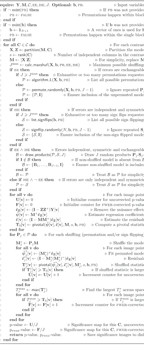
the permutations can actually be performed just by permuting the rows of the residual-forming matrixRZ. The Freedman–Lane strategy is the one used in the randomise algorithm, discussed inAppendix B.

The rationale for this permutation method is that, if the null hypoth-esis is true, thenβ= 0, and so the residuals from the reduced model with only nuisance variables,ϵZ, should not be different than the

resid-uals from the full model,ϵ, and can, therefore, be used to create the reference distribution from which p-values can be obtained.

TheSmith procedureconsists of orthogonalising the regressors of interest with respect to the nuisance variables. This is done by pre-multiplication ofXby the residual forming matrix due toZ, i.e.,RZ, then permuting this orthogonalised version of the regressors of interest. The nuisance regressors remain in the model.2

For both the Freedman–Lane and the Smith procedures, if the er-rors are independent and symmetric (ISE), the permutation matrices Pjcan be replaced for signﬂipping matricesSj. If bothEEandISEare considered appropriate, then permutation and signﬂipping can be used concomitantly.

Restricted exchangeability

Some experimental designs involve multiple observations from each subject, or the subjects may come from groups that may possess charac-teristics that may render their distributions not perfectly comparable. Both situations violate exchangeability. However, when the depen-dence between observations has a block structure, this structure can be taken into account when permuting the model, restricting the set of all otherwise possible permutations to only those that respect the re-lationship between observations (Pesarin, 2001); observations that are exchangeable only in some subsets of all possible permutations are said

weakly exchangeable(Good, 2002). TheEEandISEassumptions are then asserted at the level of these exchangeability blocks, rather than for each observation individually. The experimental hypothesis and the study design determine how theEBs should be formed and how the permuta-tion or signﬂipping matrices should be constructed. Except Huh–Jhun, the other methods inTable 2can be applied at the block level as in the unrestricted case.

Within-block exchangeability.Observations that share the same depen-dence structure, either assumed or known in advance, can be used to defineEBs such thatEEare asserted with respect to these blocks only, and the empirical distribution is constructed by permuting exclu-sively within block, as shown inFig. 2. Once the blocks have been defined, the regression of nuisance variables and the construction of the reference distribution can follow strategies as Freedman–Lane or Smith, as above. TheISE, when applicable, is transparent to this kind of block structure, so that the signflips occur as under unrestricted exchangeability. For within-block exchangeability, in general eachEB corresponds to aVG for the computation of the test statistic. See

Appendix Cfor examples.

Whole-block exchangeability.Certain experimental hypotheses may require the comparison of sets of observations to be treated as a whole, being not exchangeable within set. Exchangeability blocks can be constructed such that each include, in a consistent order, all the observations pertaining to a given set and, differently than in within-block exchangeability, here each within-block is exchanged with the others on their entirety, while maintaining the order of observations within block unaltered. ForISE, the signs areﬂipped for all observations within block at once. Variance groups are not constructed one per block; instead, eachVGencompasses one or more observations per block, all in the same order, e.g., oneVGwith theﬁrst observation of each block,

2

We name this method after Smith because, although orthogonalisation is a well known procedure, it does not seem to have been proposed by anyone to address the issues with permutation methods with theGLMuntil Smith and others presented it in a confer-ence poster (Nichols et al., 2008). We also use the eponym to keep it consistent with Ridgway (2009),and to keep the convention of calling the methods by the earliest author that we could identify as the proponent for each method, even though this method seems to have been proposed by an anonymous referee ofO'Gorman (2005).

Permutation matrix

Sign-flipping matrix

0 0 0

0 0 0 0

0 0 0

0 0 0 0 0 0 0 0 0 0 0 0 0 0

0 0 0 0

0 0 0

0 0 0 0 0 0 0 0 0 0 0 0 0 0 0 0 0 0 0

0 0

0 0 0 0 0 0 0 0 0 0 0 0 0 0 +1 +1 −1 +1 +1 −1 +1 −1 +1 Block 1 Block 2 Block 3 0 0 0 0 0 0

0 0 0

0 0 0 0 0 0 0 0 0 0 0 0

0 0 0

0 0 0 0 0 0 0 0 0 0 0 0 0 0

0 0 0

0 0

[image:6.595.314.560.549.677.2]

0 0 0 0 0 0 0 0 0 0 0 0 0 0 1 1 1 1 1 1 1 1 1 0 0 0 0 0 0 0 0 0 0

(7)

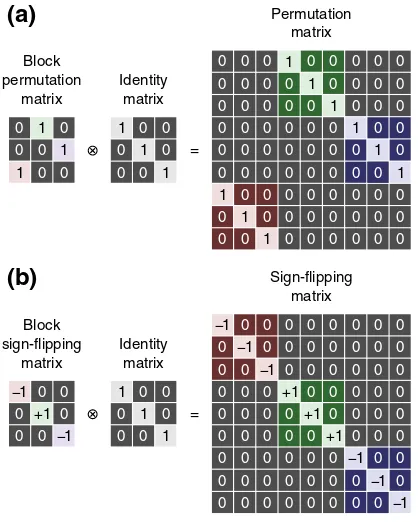
another with the second of each block and so on. Consequently, all blocks must be of the same size, and all with their observations ordered consistently, either forEEor forISE. Examples of permutation and sign

ﬂipping matrices for whole block permutation are shown inFig. 3. See

Appendix Cfor examples.

Variance groups mismatching exchangeability blocks.While variance groups can be deﬁned implicitly, as above, according to whether within- or whole-block permutation is to be performed, this is not compulsory. In some cases theEBs are deﬁned based on the non-independence between observations, even if the variances across all observations can still be assumed to be identical. SeeAppendix Cfor an example using a pairedt-test.

Choice of the conﬁguration of exchangeability blocks.The choice between whole-block and within-block is based on assumptions, or on knowl-edge about the non-independence between the error terms, as well as on the need to effectively break, at each permutation, the relationship between the data and the regressors of interest. Whole-block can be considered whenever the relationship within subsets of observations, all of the same size, is not identical, but follows a pattern that repeats it-self at each subset. Within-block exchangeability can be considered when the relationship between all observations within a subset is iden-tical, even if the subsets are not of the same size, or the relationship itself is not the same for all of them. Whole-block and within-block are straightforward ways to determine the set of valid permutations, but are not the only possibility to determine them, nor are mutually exclu-sive. Whole-block and within-block can be mixed with each other in various levels of increasing complexity.

Choice of the statistic with exchangeability blocks.All the permutation strategies discussed in the previous section can be used with virtually any statistic, the choice resting on particular applications, and constitut-ing a separate topic. The presence of restrictions on exchangeability and

variance groups reduces the choices available, though. The statisticsF

andt, described inModel and notation, are pivotal and follow known distributions when, among other assumptions, the error terms for all observations are identically distributed. Under these assumptions, all the errors terms can be pooled to compute the residual sum of squares (the term^ϵ′_^_ϵ_{in Eq.}₍₃₎_{) and so, the variance of the parameter estimates.}

This forms the basis for parametric inference, and is also useful for non-parametric tests. However, the presence ofEBs can be incompatible with the equality of distributions across all observations, with the unde-sired consequence that pivotality is lost, as shown in theResults. Al-though these statistics can still be used with permutation methods in general, the lack of pivotality for imaging applications can cause prob-lems for correction of multiple testing. When exchangeability blocks and associated variance groups are present, a suitable statistic can be computed as:

G¼

^

ψ′C C′M′WM−1C

₋1

C′ψ^

Λrankð ÞC ð6Þ

whereWis aN×Ndiagonal weighting matrix that has elementsWnn¼ ∑n′_∈g

nRn′n′ ^ϵ′

gn^ϵgn

, wheregnrepresents the variance group to which then-th

ob-servation belongs,Rn′n′ is then′-th diagonal element of the residual

forming matrix, and^ϵgn is the vector of residuals associated with the

sameVG.3_{In other words, each diagonal element of}_W_{is the reciprocal}

of the estimated variance for their corresponding group. This variance estimator is equivalent to the one proposed byHorn et al. (1975). The remaining term in Eq.(6)is given by (Welch, 1951):

Λ¼1þ2_{s s}_ððs−_þ1₂Þ_ÞX

g 1 X

n∈gRnn 1−

X n∈gWnn traceð ÞW 0

@

1 A 2

ð7Þ

[image:7.595.56.265.425.686.2]

wheres¼rank(C) as before. The statisticGprovides a generalisation of a number of well known statistical tests, some of them summarised in

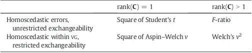
Table 3. When there is only oneVG, variance estimates can be pooled across all observations, resulting inΛ= 1 and so,G=F. IfW=V−1_, the inverse of the true covariance matrix,Gis the statistic for anF-test in a weighted least squares model (WLS) (Christensen, 2002). If there are multiple variance groups,Gis equivalent to thev2_{statistic for the} problem of testing the means for these groups under no homoscedastic-ity assumption, i.e., when the variances cannot be assumed to be all equal (Welch, 1951).4_{If, despite heteroscedasticity,}_Λ_{is replaced by 1,}

Gis equivalent to the James' statistic for the same problem (James, 1951). When rank(C) = 1, and if there are more than oneVG, sign β^

ffiffiffiffi

G

p

is the well-knownvstatistic for the Behrens–Fisher problem (Aspin and Welch, 1949; Fisher, 1935b); with only oneVGpresent, the same expression produces the Student'ststatistic, as shown earlier. If the deﬁnition of the blocks and variance groups is respected, all these particular cases produce pivotal statistics, and the generalisation pro-vided byGallows straightforward implementation.

Number of permutations

For a study withNobservations, the maximum number of possible permutations isN!, and the maximum number of possible signﬂips is 2N. However, in the presence ofBexchangeability blocks that are

0 0 0 1 1 1 0 0 0 0 1 1 0 0 1 = 0 0 0 1

0 0 0

0 0

0 0 0 0

0 0 0

0 0

0 0 0 0 0 0 0 0 0 0 0 0 0 0 0 0 0 0 0 0 0 0 0 0 0 0 1 1 0 0 1 0 0 0 1 1 1 0 0 0 0 0 0 0 0 0 0 0 0 0 0 0 0

0 0 0 0 0 0 0

1 1 0 0 0 0 1 0 0 Permutation matrix Identity matrix Block permutation matrix 0 0 0 0 1 1 0 0 1 = 0 0 0 0 0 0 −1 +1 −1

0 0 0

0 0

0 0 0 0 0 0 0

0 0

0 0 0 0 0 0 0 0 0 0 0 0 0 0 0 0 0 0 0 0 0 0 0 0 0 0 0 0 0 0 0 0 0 0 0 0 0

0 0 0 0 0 0 0

0 0 0 0 0 0 −1 −1 −1 +1 +1 +1 −1 −1 −1 0 0 0 0 0 0 0 0 0 Sign-flipping matrix Identity matrix Block sign-flipping matrix

(a)

(b)

Fig. 3.(a) Example of a permutation matrix that shuffles whole blocks of data. The blocks need to be of the same size. (b) Example of a signflipping matrix that changes the signs of the blocks as a whole. Both matrices can be constructed by the Kronecker product (represented by the symbol⊗) of a permutation or a signflipping matrix (with size determined by the number of blocks) and an identity matrix (with size determined by the number of observations per block).

3

Note that, for clarity,Gis deﬁned in Eq.(6)as a function ofM,ψandCin the unpartitioned model. With the partitioning described in theAppendix A, each of these variables is replaced by their equivalents in the partitioned, full model, i.e., [X Z], [β′γ′]′ and [Is×s0s× (r−s)]′respectively.

4

(8)

exchangeable as a whole, the maximum number of possible permuta-tions drops to no more thanB!, and the maximum number of sign

ﬂips to 2B_{. For designs where data is only exchangeable within-block,}

the maximum number of possible permutations is∏bB= 1Nb!, where

Nbis the number of observations for theb-th block, and the maximum

number of signﬂips continues to be 2N_.

[image:8.595.42.294.77.130.2]

However, the actual number of possible rearrangements may be smaller depending on the null hypothesis, the permutation strategy, or other aspects of the study design. If there are discrete covariates, or if there are ties among continuous regressors, many permutations may not alter the model at all. The maximum number of permutations can be calculated generically from the design matrix observing the number of repeated rows among the regressors of interest for the Freedman–Lane and most other methods, or inMfor the ter Braak and Manly methods. The maximum number of possible permutations or signﬂips, for different restrictions on exchangeability, is shown in

Table 4.

Even considering the restrictions dictated by the study design, the number of possible shufflings tends to be very large, even for samples of moderate size, and grows very rapidly as observations are included. When the number of possible rearrangements is large, not all of them need to be performed for the test to be valid (Chung and Fraser, 1958; Dwass, 1957), and the resulting procedure will be approximately exact (Edgington, 1969). The number can be chosen according to the availability of computational resources and considerations about power and precision. The smallest p-value that can be obtained con-tinues to be 1/J, whereJis the number of permutations performed. The precision of permutation p-values may be determined considering the confidence interval around the significance level.

To efﬁciently avoid permutations that do not change the design ma-trix, the Algorithm“L”(Knuth, 2005) can be used. This algorithm is sim-ple and has the beneﬁt of generating only permutations that are unique,

i.e., in the presence of repeated elements, it correctly avoids synony-mous permutations. This is appropriate when enumerating all possible permutations. However, the algorithm produces sequentially permuta-tions that are in lexicographic order. Although this can be advantageous in other settings, here this behaviour can be problematic when running only a subset of_P, and has the potential to bias the results. For imaging applications, where there are many points (voxels, vertices, faces) being analysed, it is in general computationally less expensive to shuffle many times a sequence of values and store these permuted sequences, than actuallyfit the permuted model for all points. As a consequence, the problem with lexicographically ordered permutations can be solved by generating all the possible permutations, and randomly drawingJ el-ements fromPto do the actual shufflings of the model, or generating random permutations and checking for duplicates. Alternatively, the procedure can be conducted without attention to repeated permuta-tions using simple shuf_fling of the data. This strategy is known as condi-tional Monte Carlo(CMC) (Pesarin and Salmaso, 2010; Trotter and Tukey, 1956), as each of the random realisations is conditional on the available observed data.

Signflipping matrices, on the other hand, can be listed using a numeral system with radix 2, and the signflipped models can be performed without the need to enumerate all possibleflips or to appeal toCMC. The simplest strategy is to use the digits 0 and 1 of the binary numeral system, treating 0 as−1 when assembling the matrix. In a binary system, each signflipping matrix is also its own numerical identifier, such that avoiding repeated signflippings is trivial. The binary representation can be converted to and from radix 10 if needed, e.g., to allow easier human readability.

For within-block exchangeability, permutation matrices can be con-structed within-block, then concatenated along their diagonal to assem-blePj, which also has a block structure. The elements outside the blocks

are_filled with zeros as needed (Fig. 2). The block de_finitions can be ignored for signflipping matrices for designs whereISEis asserted within-block. For whole-block exchangeability, permutation and sign

ﬂipping matrices can be generated by treating each block as an element, and theﬁnalPjorSjare then assembled via Kronecker multiplication by

an identity matrix of the same size as the blocks (Fig. 3).

Multiple testing

Differently than with parametric methods, correction for multiple testing using permutation does not require the introduction of more as-sumptions. For familywise error rate correction (FWER), the method was described byHolmes et al. (1996). As the statisticsTj∗are calculated for

each shufﬂing to build the reference distribution at each point, the max-imum value ofTj∗across the image,Tjmax, is also recorded for each

rear-rangement, and its empirical distribution is obtained. For each test in the image, anFWER-corrected p-value can then be obtained by comput-ing the proportion ofTjmaxthat is aboveT0for each test. A singleFWER threshold can also be applied to the statistical map ofT0values using the distribution ofTjmax. The same strategy can be used for statistics

that combine spatial extent of signals, such as cluster extent or mass (Bullmore et al., 1999), threshold-free cluster enhancement (TFCE) (Smith and Nichols, 2009) and others (Marroquin et al., 2011). For these spatial statistics, the effect of lack of pivotality can be mitigated by non-stationarity correction (Hayasaka et al., 2004; Salimi-Khorshidi et al., 2011).

The p-values under the null hypothesis are uniformly distributed in the interval [0,1]. As a consequence, the p-values themselves are pivotal quantities and, in principle, could be used for multiple testing correction as above. The distribution of minimum p-value,pjmin, instead ofTjmax, can

be used. Due to the discreteness of the p-values, this approach, however, entails some computational difﬁculties that may cause considerable loss of power (Pantazis et al., 2005). Correction based on false-discovery rate (FDR) can be used once the uncorrected p-values have been obtained for each point in the image. Either a singleFDRthreshold can be applied to Table 3

The statisticGprovides a generalisation for a number of well known statistical tests.

rank(C) = 1 rank(C)N1 Homoscedastic errors,

unrestricted exchangeability

Square of Student'st F-ratio

Homoscedastic withinVG, restricted exchangeability

[image:8.595.43.293.551.662.2]

Square of Aspin–Welchv Welch'sv2

Table 4

Maximum number of unique permutations considering exchangeability blocks.

Exchangeability EE ISE

Unrestricted N! 2N

Unrestricted, repeated rows N!∏M m¼1

1

Nm! 2N

Within-block ∏B

b¼1

Nb! 2N

Within-block, repeated rows ∏B b¼1

Nb!M∏jb m¼1

1 Nmjb!

2N

Whole-block B! 2B

Whole-block, repeated blocks B!∏eM e m¼1

1

N_e_m! 2

B

BNumber of exchangeability blocks (EB). MNumber of distinct rows inX.

M|bNumber of distinct rows inXwithin theb-th block. e

MNumber of distinct blocks of rows inX. NNumber of observations.

NbNumber of observations in theb-th block.

NmNumber of times each of theMdistinct rows occurs inX.

(9)

the map of uncorrected p-values (Benjamini and Hochberg, 1995; Genovese et al., 2002) or anFDR-adjusted p-value can be calculated at each point (Yekutieli and Benjamini, 1999).

Evaluation methods

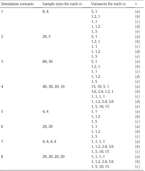
We conducted extensive simulations to study the behaviour of the commonFstatistic (Eq.3) as well as of the generalisedGstatistic (Eq.6), proposed here for use in neuroimaging, in various scenarios of balanced and unbalanced designs and variances for the variance groups. Some of the most representative of these scenarios are shown inTable 5. The main objective of the simulations was to assess whether these sta-tistics would retain their distributions when the variances are not equal for each sample. Within each scenario, 3 or 5 different conﬁgurations of simulated variances were tested, pairwise, for the equality of distribu-tions using the two-sample Kolmogorov–Smirnov test (KS) (Press et al., 1992), with a signiﬁcance levelα= 0.05, corrected for multiple testing within each scenario using the Bonferroni correction, as these tests are independent.

For each variance configuration, 1000 voxels containing normally distributed random noise, with zero expected mean, were simulated and tested for the null hypothesis of no difference between the means of the groups. The empirical distribution of the statistic for each confi g-uration was obtained by pooling the results for the simulated voxels, then compared with theKStest. The process was repeated 1000 times, and the number of times in which the distributions were found to be significantly different from the others in the same scenario was

recorded. Conﬁdence intervals (95%) were computed using the Wilson method (Wilson, 1927).

By comparing the distributions of the same statistic obtained in different variance settings, this evaluation strategy mimics what is observed when the variances for each voxel varies across space in the same imaging experiment, e.g.,(a),(b)and(c)inTable 5could be different voxels in the same image. The statistic must be robust to these differences and retain its distributional properties, even if assessed non-parametrically, otherwiseFWERusing the distribution of the maximum statistic is compromised. The same applies to multiple testing that combines more than one imaging modality.

In addition, the same scenarios and variance configurations were used to assess the proportion of error typeIand the power of theF andGstatistics. To assess power, a simulated signal was added to each of the groups; for the scenarios with two groups, the trueψwas defined as [0 -1]_′, whereas for the scenarios with four groups, it was de_fined as [0 -0.33 -0.67 -1]′. In either case, the null hypothesis was that the group means were all equal. Significance values were computed using 1000 permutations, with_α= 0.05, and 95% con_fidence intervals were calculated using the Wilson method.

Permutation strategies

We compared the 10 methods described inTable 2simulating differ-ent regression scenarios. The design considered one regressor of inter-est,x1, and two regressors of no interest,z1andz2,z2being a column-vector of just ones (intercept). The simulation scenarios considered different sample sizes,N= {12, 24, 48, 96}; different combinations for continuous and categoricalx1andz1; different degrees of correlation betweenx1andz1,ρ= {0, 0.8}; different sizes for the regressor of interest,_β1= {0, 0.5}; and different distributions for the error terms,

ϵ, as normal (μ= 0,σ2_{= 1), uniform}h₋p₃ffiffiffi_;_þpffiffiffi₃i_{, exponential} (λ= 1) and Weibull (λ= 1,k= 1/3). The coefficients for thefirst regres-sor of no interest and for the intercept were kept constant asγ1= 0.5 andγ2= 1 respectively, and the distributions of the errors were shifted or scaled as needed to have expected zero mean and expected unit variance.

The continuous regressors were constructed as a linear trend rang-ing from−1 to +1 forx1, and the square of this trend, mean-centred, forz1. For this symmetric range around zero forx1, this procedure causesx1and z1to be orthogonal and uncorrelated. For the discrete regressors, a vector ofN/2 ones andN/2 negative ones was used, the

firstN/2 values being only + 1 and the remaining−1 forx1, whereas forz1, thefirst and lastN/4 were−1 and theN/2 middle values were +1. This procedure also causesx1andz1to be orthogonal and uncorre-lated. For each different configuration, 1000 simulated vectorsYwere constructed asY= [x1z1z2][β1γ1γ2]′+ϵ.

Correlation was introduced in the regression models through Cholesky decomposition of the desired correlation matrixK, such thatK=L′L, then defining the regressors by multiplication byL, i.e., [x1ρ z1ρ] = [x1z1]L. The unpartitioned design matrix was con-structed asM= [x1ρz1ρz2]. A contrastC= [1 0 0]′was defined to test the null hypothesisH ¼0:C′ψ=β1= 0. This contrast tests only thefirst column of the design matrix, so partitioningM= [X Z] using the scheme shown inAppendix Amight seem unnecessary. However, we wanted to test also the effect of non-orthogonality between columns of the design matrix for the different permutation methods, with and without the more involved partitioning scheme shown in the Appendix. Using a single variance configuration across all observations in each simulation, modelling a single variance group, and with rank(C) = 1, the statistic used was the Student'st(Table 3), a particular case of the

[image:9.595.38.287.447.740.2]

Gstatistic. Permutation, signflipping, and permutation with signfl ip-ping were tested. Up to 1000 permutations and/or signflippings were performed usingCMC, being less when the maximum possible number Table 5

The eight different simulation scenarios, each with its own same sample sizes and different variances. The distributions of the statistic (ForG) for each pair of variance conﬁguration within scenario were compared using the KS test. The letters in the last col-umn (marked with a star,⋆) indicate the variance conﬁgurations represented in the pairwise comparisons shown inFig. 4and results shown inTable 6.

Simulation scenario Sample sizes for eachVG Variances for eachVG ⋆

1 8, 4 5, 1 (a)

1.2, 1 (b)

1, 1 (c)

1, 1.2 (d)

1, 5 (e)

2 20, 5 5, 1 (a)

1.2, 1 (b)

1, 1 (c)

1, 1.2 (d)

1, 5 (e)

3 80, 30 5, 1 (a)

1.2, 1 (b)

1, 1 (c)

1, 1.2 (d)

1, 5 (e)

4 40, 30, 20, 10 15, 10, 5, 1 (a)

3.6, 2.4, 1.2, 1 (b) 1, 1, 1, 1 (c) 1, 1.2, 2.4, 3.6 (d) 1, 5, 10, 15 (e)

5 4, 4 1, 1 (a)

1, 1.2 (b)

1, 5 (c)

6 20, 20 1, 1 (a)

1, 1.2 (b)

1, 5 (c)

7 4, 4, 4, 4 1, 1, 1, 1 (a)

1, 1.2, 2.4, 3.6 (b) 1, 5, 10, 15 (c)

8 20, 20, 20, 20 1, 1, 1, 1 (a)

(10)

of shufﬂings was not large enough. In these cases, all the permutations and/or signﬂippings were performed exhaustively.

Error typeIwas computed usingα= 0.05 for conﬁgurations that used

β1= 0. The other conﬁgurations were used to examine power. As previ-ously, conﬁdence intervals (95%) were estimated using the Wilson method.

Results

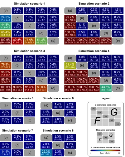
Fig. 4shows heatmaps with the results of the pairwise comparisons between variance conﬁgurations, within each of the simulation

scenarios presented inTable 5, using eitherForGstatistic. For unbal-anced scenarios with only two samples (simulation scenarios 1 to 3), and with modest variance differences between groups (con_ﬁgurations

[image:10.595.104.505.198.701.2]

btod), theFstatistic often retained its distributional properties, albeit less often than theGstatistic. For large variance differences, however, this relative stability was lost forF, but not forG(aande). Moreover, the inclusion of more groups (scenario 4), with unequal sample sizes, caused the distribution of theFstatistic to be much more sensitive to heteroscedasticity, such that almost always theKStest identiﬁed differ-ent distributions across differdiffer-ent variance conﬁgurations. TheGstatistic, on the other hand, remained robust to heteroscedasticity even in these cases. As one of our reviewers highlighted, a variance ratio of 15:1 (as

(11)

used in Scenarios 4, 7 and 8) may seem somewhat extreme, but given the many thousands, often millions, of voxels in an image, it is not un-reasonable to suspect that such large variance differences may exist across at least some of them.

In balanced designs, either with two (simulation scenarios 5 and 6) or more (scenarios 7 and 8) groups, theFstatistic had a better behaviour than in unbalanced cases. For two samples of the same size, there is no difference betweenFandG: both have identical values and produce the same permutation p-values.5_{For more than two groups, the}_G_statistic

behaved consistently better thanF, particularly for large variance differences.

These results suggest that theGstatistic is more appropriate under heteroscedasticity, with balanced or unbalanced designs, as it preserves its distributional properties, indicating more adequacy for use with neuroimaging. TheFstatistic, on the other hand, does not preserve pivotality but can, nonetheless, be used under heteroscedasticity when the groups have the same size.

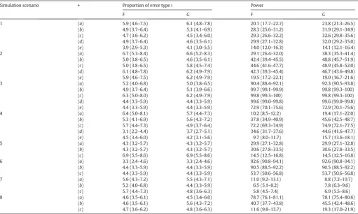
With respect to error typeI, both FandG resulted in similar amount of false positives when assessed non-parametrically. TheG

yielded generally higher power thanF, particularly in the presence of heteroscedasticity and with unequal sample sizes. These results are presented inTable 6.

Permutation strategies

The different simulation parameters allowed 1536 different regres-sion scenarios, being 768 without signal and 768 with signal; a summa-ry is shown inTable 7, and some of the most representative inTable 8. In “well behaved”scenarios, i.e., large number of observations, orthogonal regressors and normally distributed errors, all methods tended to behave generally well, with adequate control over typeIerror and fairly similar power. However, performance differences between the permu-tation strategies shown inTable 2became more noticeable as the sample sizes were decreased and skewed errors were introduced.

Some of the methods are identical to each other in certain circum-stances. IfXandZare orthogonal, Draper–Stoneman and Smith are equivalent. Likewise under orthogonality, Still–White produces identi-cal regression coefﬁcients as Freedman–Lane, although the statistic will only be the same if the loss in degrees of freedom due toZis taken into account, something not always possible when the data has already been residualised and no information about the original nuisance variables is available. Nonetheless, the two methods remain asymptotically equivalent as the number of observations diverges from the number of nuisance regressors.

Sample size

Increasing the sample size had the effect of approaching the error rate closer to the nominal levelα= 0.05 for all methods in virtually all parameter conﬁgurations. For small samples, most methods were slightly conservative, whereas Still–White and Kennedy were anti-conservative and often invalid, particularly if the distributions of the errors were skewed.

5

[image:11.595.40.551.85.391.2]

Parametric p-values for these two statistics, however, differ. If computed, parametric p-values would have to consider that the degrees of freedom for theGstatistic are not the same as forF; see footnote 4.

Table 6

Proportion of error type I and power (%) for the statisticsFandGin the various simulation scenarios and variance conﬁgurations shown inTable 5. Conﬁdence intervals (95%) are shown in parenthesis.

Simulation scenario ⋆ Proportion of error typeI Power

F G F G

1 (a) 5.9 (4.6–7.5) 6.1 (4.8–7.8) 20.1 (17.7–22.7) 23.8 (21.3–26.5)

(b) 4.9 (3.7–6.4) 5.3 (4.1–6.9) 28.3 (25.6–31.2) 31.9 (29.1–34.9) (c) 4.7 (3.6–6.2) 4.5 (3.4–6.0) 29.3 (26.6–32.2) 32.6 (29.8–35.6) (d) 4.9 (3.7–6.4) 4.6 (3.5–6.1) 29.9 (27.1–32.8) 32.0 (29.2–35.0) (e) 3.9 (2.9–5.3) 4.1 (3.0–5.5) 14.0 (12.0–16.3) 14.1 (12.1–16.4)

2 (a) 6.7 (5.3–8.4) 6.6 (5.2–8.3) 29.1 (26.4–32.0) 38.3 (35.3–41.4)

(b) 5.0 (3.8–6.5) 4.6 (3.5–6.1) 42.4 (39.4–45.5) 48.8 (45.7–51.9) (c) 5.0 (3.8–6.5) 5.8 (4.5–7.4) 44.6 (41.6–47.7) 48.9 (45.8–52.0) (d) 6.1 (4.8–7.8) 6.2 (4.9–7.9) 42.3 (39.3–45.4) 46.7 (43.6–49.8) (e) 5.9 (4.6–7.5) 6.2 (4.9–7.9) 19.5 (17.2–22.1) 19.0 (16.7–21.6)

3 (a) 5.2 (4.0–6.8) 5.0 (3.8–6.5) 90.4 (88.4–92.1) 92.3 (90.5–93.8)

(b) 4.9 (3.7–6.4) 5.1 (3.9–6.6) 99.7 (99.1–99.9) 99.8 (99.3–100)

(c) 6.3 (5.0–8.0) 6.2 (4.9–7.9) 99.8 (99.3–100) 99.8 (99.3–100)

(d) 4.4 (3.3–5.9) 4.4 (3.3–5.9) 99.6 (99.0–99.8) 99.6 (99.0–99.8) (e) 4.4 (3.3–5.9) 4.4 (3.3–5.9) 72.9 (70.1–75.6) 72.9 (70.1–75.6)

4 (a) 6.4 (5.0–8.1) 5.7 (4.4–7.3) 10.2 (8.5–12.2) 19.4 (17.1–22.0)

(b) 5.3 (4.1–6.9) 5.6 (4.3–7.2) 37.8 (34.9–40.9) 45.6 (42.5–48.7) (c) 5.7 (4.4–7.3) 4.9 (3.7–6.4) 72.2 (69.3–74.9) 74.9 (72.1–77.5) (d) 3.1 (2.2–4.4) 3.7 (2.7–5.1) 34.6 (31.7–37.6) 44.6 (41.6–47.7)

(e) 4.5 (3.4–6.0) 4.2 (3.1–5.6) 9.7 (8.0–11.7) 15.7 (13.6–18.1)

5 (a) 4.3 (3.2–5.7) 4.3 (3.2–5.7) 29.9 (27.1–32.8) 29.9 (27.1–32.8)

(b) 4.3 (3.2–5.7) 4.3 (3.2–5.7) 30.6 (27.8–33.5) 30.6 (27.8–33.5) (c) 6.9 (5.5–8.6) 6.9 (5.5–8.6) 14.5 (12.5–16.8) 14.5 (12.5–16.8)

6 (a) 3.3 (2.4–4.6) 3.3 (2.4–4.6) 92.6 (90.8–94.1) 92.6 (90.8–94.1)

(b) 4.4 (3.3–5.9) 4.4 (3.3–5.9) 90.5 (88.5–92.2) 90.5 (88.5–92.2) (c) 4.4 (3.3–5.9) 4.4 (3.3–5.9) 53.7 (50.6–56.8) 53.7 (50.6–56.8)

7 (a) 5.6 (4.3–7.2) 5.5 (4.3–7.1) 11.0 (9.2–13.1) 8.8 (7.2–10.7)

(b) 5.2 (4.0–6.8) 4.4 (3.3–5.9) 6.5 (5.1–8.2) 7.8 (6.3–9.6)

(c) 5.7 (4.4–7.3) 4.8 (3.6–6.3) 5.8 (4.5–7.4) 6.9 (5.5–8.6)

8 (a) 4.6 (3.5–6.1) 4.5 (3.4–6.0) 78.7 (76.1–81.1) 78.1 (75.4–80.6)

(b) 4.6 (3.5–6.1) 5.6 (4.3–7.2) 40.7 (37.7–43.8) 45.5 (42.4–48.6)

(12)

Continuous or categorical regressors of interest

For all methods, using continuous or categorical regressors of inter-est did not produce remarkable differences in the observed proportions of typeIerror, except if the distribution of the errors was skewed and signﬂipping was used (in violation of assumptions), in which case Manly and Huh_–Jhun methods showed erratic control over the amount of errors.

Continuous or categorical nuisance regressors

The presence of continuous or categorical nuisance variables did not substantially interfere with either control over error typeIor power, for any of the methods, except in the presence of correlated regressors.

Degree of non-orthogonality and partitioning

All methods provided relatively adequate control over error typeI in the presence of a correlated nuisance regressor, except Still_– White (conservative) and Kennedy (inﬂated rates). The partitioning scheme mitigated the conservativeness of the former, and the anti-conservativeness of the latter.

Distribution of the errors

Different distributions did not substantially improve or worsen error rates when using permutation alone. Still–White and Kennedy tended to fail to control error typeIin virtually all situations. Signﬂipping alone, when used with asymmetric distributions (in violation of as-sumptions), required larger samples to allow approximately exact con-trol over the amount of error typeI. In these cases, and with small samples, the methods Draper–Stoneman, Manly and Huh–Jhun tended to display erratic behaviour, with extremes of conservativeness and anticonservativeness depending on the other simulation parameters. The same happened with the parametric method. Freedman–Lane and Smith methods, on the other hand, tended to have a relatively constant and somewhat conservative behaviour in these situations. Permutation combined with signﬂipping generally alleviated these issues where they were observed.

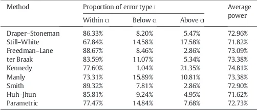
[image:12.595.42.293.137.245.2]

From all the methods, the Freedman_–Lane and Smith were those that performed better in most cases, and with their 95% conﬁdence interval covering the desired error level of 0.05 more often than any of the other methods. The Still–White and Kennedy methods did not generally control the error typeIfor most of the simulation parameters, particularly for smaller sample sizes. On the other hand, with a few exceptions, the Freedman–Lane and the Smith methods effectively controlled the error rates in most cases, even with skewed errors and signﬂipping, being, at worst, conservative or only slightly above the nominal level. All methods were, overall, Table 7

A summary of the results for the 1536 simulations with different parameters. The amount of error type I is calculated for the 768 simulations without signal (β1= 0). Conﬁdence intervals (CI) at 95% were computed around the nominal levelα= 0.05, and the observed amount of errors for each regression scenario and for each method was compared with this interval. Methods that mostly remain within the CI are the most appropriate. Methods that frequently produce results below the interval areconservative; those above areinvalid. Power was calculated for the remaining 768 simulations, which contained signal (β1= 0.5).

Method Proportion of error typeI Average power WithinCI BelowCI AboveCI

Draper–Stoneman 86.33% 8.20% 5.47% 72.96% Still–White 67.84% 14.58% 17.58% 71.82% Freedman–Lane 88.67% 8.46% 2.86% 73.09%

ter Braak 83.59% 11.07% 5.34% 73.38%

Kennedy 77.60% 1.04% 21.35% 74.81%

Manly 73.31% 15.89% 10.81% 73.38%

Smith 89.32% 7.81% 2.86% 72.90%

Huh–Jhun 85.81% 9.24% 4.95% 71.62%

Parametric 77.47% 14.84% 7.68% 72.73%

Table 8

Proportion of error type I (fora= 0.05), for some representative of the 768 simulation scenarios that did not have signal, using the different permutation methods, and withGas the sta-tistic in the absence of EB (so, equivalent to theFstatistic). Conﬁdence intervals (95%) are shown in parenthesis.

Simulation parameters Proportion of error typeI(%)

N x1 z1 ρ ϵ EE ISE D–S S–W F–L tB K M S H–J P

[image:12.595.46.562.472.710.2]