A first catalogue of automatically selected ultraviolet excess sources from the UVEX survey

University of Warwick institutional repository: http://go.warwick.ac.uk/wrap

This paper is made available online in accordance with

publisher policies. Please scroll down to view the document

itself. Please refer to the repository record for this item and our

policy information available from the repository home page for

further information.

To see the final version of this paper please visit the publisher’s website.

Access to the published version may require a subscription.

Author(s): Kars Verbeek, Eelco de Groot, Paul J. Groot, Simone

Scaringi, Janet Drew, Robert Greimel, Mike Irwin, Eduardo

González-Solares, Boris T. Gänsicke, Jorge Casares, Jesus M. Corral-Santana,

Niall Deacon, Danny Steeghs

Article Title: A first catalogue of automatically selected

ultraviolet-excess sources from the UVEX survey

Year of publication: 2012

Link to published article:

http://link.aps.org/doi/10.1111/j.1365-2966.2011.20094.x

Publisher statement: ‘The definitive version is

arXiv:1111.0440v1 [astro-ph.GA] 2 Nov 2011

A first catalogue of automatically selected UV-excess

sources from the UVEX survey

Kars Verbeek

, Eelco de Groot

, Paul J. Groot

, Simone Scaringi

, Janet Drew

,

Robert Greimel

, Mike Irwin

, Eduardo Gonz´

alez-Solares

, Boris T. G¨

ansicke

,

Jorge Casares

, Jesus M. Corral-Santana

, Niall Deacon

and Danny Steeghs

1_{Department of Astrophysics, Radboud University Nijmegen, P.O. Box 9010, 6500 GL Nijmegen, The Netherlands}

2_{Centre for Astronomy Research, Science & Technology Research Institute, University of Hertfordshire, Hatfield, AL10 9AB, UK} 3_{Institut f¨ur Physik, Karl-Franzen Universit¨at Graz, Universit¨atsplatz 5, 8010 Graz, Austria}

4_{Cambridge Astronomy Survey Unit, Institute of Astronomy, University of Cambridge, Madingley Road, Cambridge, CB3 0HA, UK} 5_{Physics Department, University of Warwick, Coventry, CV4 7AL, UK}

6_{Instituto de Astrof´ısica de Canarias, Via Lactea, s/n E-38205 La Laguna (Tenerife), Spain}

7_{Departamento de Astrof´ısica, Universidad de La Laguna, La Laguna E-38205, S/C de Tenerife, Spain} 8_{Institute for Astronomy, University of Hawaii, 2680 Woodlawn Drive, Honolulu, HI 96822, USA}

Accepted ... Received ...; in original form ...

ABSTRACT

We present the first catalogue of point-source UV-excess sources selected from the UVEX_survey.UVEX_{images the Northern Galactic Plane in the}U, g, rand Heiλ5875 bands in the Galactic latitude range –5◦_{< b <+5}◦_{. Through an automated algorithm,}

which works on a field-to-field basis, we select blue UV-excess sources in 211 square degrees from the (U₋g) vs. (g₋r) colour-colour diagram and thegvs. (U₋g) andg vs. (g−r) colour-magnitude diagrams. The UV-excess catalogue covers the magnitude

range 14< g <22.5, contains 2 170 sources and consists of a mix of white dwarfs, post-common-envelope objects, interacting binaries, quasars and AGN. Two other samples of outliers were found during the selection: i) a ‘subdwarf’ sample, consisting of no less than 9 872 candidate metal-poor stars or lightly reddened main-sequence stars, and ii) a ‘purple’ sample consisting of 803 objects, most likely a mix of reddened late M-giants, T Tauri stars, planetary nebulae, symbiotic stars and carbon stars. Cross-matching the selected UV-excess catalogue with other catalogues aids with the first classification of the different populations and shows that more than 99% of our selected sources are unidentified sources.

Key words: surveys – stars:general – ISM:general – Galaxy: stellar content – Galaxy:

disc – Galaxy:structure

1 INTRODUCTION

The UV-excess survey of the Northern Galactic Plane (UVEX₎1 _{images a strip of 10×185 degrees (–5}◦

< b <+5◦_{) along the Northern Galactic plane in theU, g, rand}

He_iλ5875 bands down to ∼21st

−22nd _{magnitude using}

the Wide Field Camera mounted on the Isaac Newton Telescope, on the island of La Palma. The spatial pixel scale is 0.33 arcsec/pixel with a field of view of 0.29 square degree per pointing. The exposure times are 30 seconds for the r- and g-band images, 120 seconds for theU-band images and 180 seconds for the Heiλ5875-band images. A

full description of the survey is given in Groot et al. (2009;

⋆ _{E-mail:[email protected]} 1 _{http://www.uvexsurvey.org}

hereafter G09).

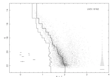
Figure 1. gvs. (g−_r) colour-magnitude diagram of field UVEX 6162 (_l=80.76, _b= –1.90). Data shown are all stellar and probably stellar detections in ther- andg-bands with a photometric error smaller than 0.1 magnitudes in these bands. The solid lines show our automated selection technique and the outline of the (g−_r) colour at which the_g-band magnitude peaks (right, thick line), and the 3_σ limit for eachg-band magnitude bin (left thin line), called the ‘blue edge’. All sources more than 3 times their own photometric error to the left of this blue edge are selected (here plotted with their own photometric errors). The error bars on the right side show the average photometric error in (g−_r) per bin.

neutron star and black hole binaries. Our understanding of these populations is often limited due to the small number of known systems and/or strong selection biases in known samples (see e.g. Pretorius, Knigge & Kolb, 2007).

Traditionally blue/UV surveys, targeting quasars and AGN, specifically concentrate on higher Galactic latitudes to avoid the problems of crowding and dust extinction. The post-common-envelope objects mentioned above are generally hot but intrinsically faint so their absolute visual magnitudes are several magnitudes lower than main-sequence stars with similar colours. In the plane of the Milky Way an intrinsically blue, low-luminosity population of objects is visible in theg vs. (U−g) and g vs. (g−r) colour-magnitude diagrams as UV-excess sources against a background of higher luminosity, more distant and therefore more highly reddened, objects. Examples of colour-magnitude diagrams and colour-colour diagrams showing this effect are shown in G09 (Figs. 13 and 14) and Figs. 1 and 2 above.

It is our aim to distinguish UV-excess sources from the normal main-sequence stars in a user-independent way and we have therefore developed an automated selection technique to construct our catalogue, presented in Sect.

2. In Sect. 3 we apply this selection technique to the UVEXdata of 211 square degrees and analyse the spatial, magnitude and colour distributions of the UV-excess sources selected from this area. In Sect. 4 we classify the UV-excess sources making use of the IPHAS_{database, cross-matches} to Simbad and synthetic colours of stellar populations as presented in G09 and Drew et al. (2005). Finally in Sect. 5 we summarize the results and conclusions of our selection algorithm and catalogue of UV-excess candidates.

Figure 2.gvs. (U−_g) colour-magnitude diagram of field UVEX 6162. The solid lines show our automated selection technique and the outline of the (U−_g) colour at which the_g-band magnitude peaks (right, thick line), and the 3_σlimit for each_g-band magnitude bin (left thin line), called the ‘blue edge’. All sources more than 3 times their own photometric error to the left of this blue edge are selected. Not all sources plotted with their own photometric errors here were selected in this colour-magnitude diagram: the two blue sources fainter thang=21 are are less than 3 times their own photometric error to the left of the blue edge. The error bars on the right side show the average photometric error in (U−_g) per bin.

• For eachUVEX_{pointing we construct a gvs. (g−r)} and g vs. (U − g) colour-magnitude diagram (Figs. 1 and 2) and a (U −g) vs. (g−r) colour-colour diagram (Fig. 3) using all stellar and probably stellar objects with a photometric error <0.1 magnitudes (see Gonz´ alez-Solares et al., 2008 for the classification of sources within the IPHAS_andUVEX_{surveys). Each object has to be detected} twice per filter band: in a direct field and in an offset field (not necessarily the offset field belonging to the direct field).

• In thegvs. (g−r) andgvs. (U−g) colour-magnitude diagrams the main locus of objects, containing mainly reddened main-sequence stars and giants, and the selection boundary at the blue side of the main locus are determined in the following steps:

a) All objects detected in the r- and g-band images are divided in g-band magnitude bins. The width of the g-magnitude bins and the number of bins depend on the surface density of objects in the field. The total number of bins for a field isNbins=1₃

√

Ns, withNsthe total number

of selected objects in the field. The width (∆g) of a given bin is determined by sorting of the objects in such a way that for all bins the product (∆g×ns) is approximately

constant, with ns the number of objects in the given bin.

The differences in this product between the different bins

is minimized in an iterative process where two sources are added from neighbouring bins to the bin in which the product (∆g×ns) is the smallest, and one source is taken

from the bin where this product is the largest by shifting the boundary between two bins. This is repeated until the differences in the product (∆g×ns) is minimized. This

procedure is a compromise between using small bins that allow for a precise following of the main locus and using many objects per bin which suppresses statistical noise. b) The colour (in (g−r) or (U−g)) at which the distribution of objects peaks for each g-magnitude bin is calculated. This peak is found in an iterative process. Perg-magnitude bin a sliding window over the colour distribution is used to determine the smallest window in colour that contains 50% of the sources. The sample of sources within this window is again searched for the smallest sub-window that contain 50% of the sources (i.e. 25% of the original totalns). This

Figure 3.(U−_g) vs. (_g−_r) colour-colour diagram of field UVEX 6162. Data shown are all sources with a stellar or probably stellar detection in ther- andg-bands and with a photometric error smaller than 0.1 magnitudes in these bands. The lines are line fitted to the main locus (central line) and the 3σbox containing the bulk of the objects.

c) In eachg-magnitude bin the root-mean-square deviation for the objects that lie to the blue of the peak is calculated using a double pass 3-sigma-clipping. For each bin a Gaus-sian distribution in (g−r) or (U−g) is assumed centred on the peak value found in step (b). The red side of the distribution is not taken into account since the distribution here is intrinsically wider and does not show a clear cut off, as can be seen in Fig. 1. The blue edge of the main locus is now placed at three times the root-mean-square deviation to the blue of the peak value. This determines the final selection boundary or ‘blue edge’. This is the left, ‘ragged’ line in Figs. 1 and 2.

• In the g vs. (U −g) and/or g vs. (g−r) colour-magnitude diagrams, sources located more than three times their own photometric error to the left of the blue edge are selected.

• An additional selection is made in the (U −g) vs. (g−r) colour-colour diagram. The average position of the bulk of all objects is found by least-square fitting a straight line to the distribution of all selected sources. This line is broadened to a rectangular box containing the bulk of the objects (see Fig. 3). The fitting of this line and the broadening of this line to a selection box is done in a number of steps:

a) The average (g−r) and (U −g) colours of all selected objects are calculated. The 25% of sources that lie furthest

0 20 40 60 80 100 120 140 160

-3 -2.5 -2 -1.5 -1 -0.5 0 0.5 1

No of sources

projected colour

UVEX 6162

0 2 4 6 8 10

-3 -2.5 -2 -1.5 -1

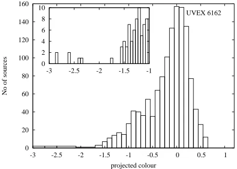
Figure 4.Histogram of projected colours parallel to the fit line of Fig.3 for field UVEX 6162. The upper left side of the rectangular selection box in the colour-colour diagram of Fig.3 is defined as the last gap in the first 10% of the data projected along the main locus. Six UV-excess sources are on the blue side of this last gap at ‘projected colour’−1_.75 to−2_.35.

away in both colours from this average (g−r),(U −g) position is temporarily discarded from the colour-colour diagram.

0 500 1000 1500 2000 0 0.2 0.4 0.6 0.8 1 1.2 1.4

No of sources

(g-r) from blue edge

Figure 5. The distribution of distances in (g−_r) magnitudes from the blue edge for objects selected from the 211 square de-grees shows two populations: a UV-excess sample (blue) and a ‘subdwarf’ sample (red) separated at a distance of 0.4 magnitudes from the blue edge. The tails of these two populations partly over-lap since the UV-excess sources at a distance less than 0.4 (g−_r) magnitudes from the blue edge are at a distance more than 0.4 (U−_g) magnitudes from the blue edge in the_gvs. (_U−_g) colour-magnitude diagram.

squares to the remaining 75% of data points. Photometric error bars on the data points are not considered at this stage to prevent the bright stars on the blue side of the main-sequence dominating the entire fit.

c) The standard deviation (σ), perpendicular to the straight line fitted to the main stellar locus, is cal-culated. Each data points has a shortest distance p

((∆(g−r))2_{+ (∆(U−g))}2_{) to the fit line, where}

∆(g−r) and ∆(U −g) are the differences in (g−r) and (U −g) colours between the fit line and the data point. We calculate σ as the average of the squared differences between the fit line and all data points. Here the 25% discarded in the previous step is included again. This standard deviation is used for a sigma cut at 2σ (a cut at 3σ would discard too many main-sequence sources). After this sigma cut most main-sequence stars and UV-excess sources are still included in the sample, but most objects both blue in (U−g) and red in (g−r) are excluded. d) A new straight line is fitted using the standard least-square method to the remaining data after the 2σ cut of step (c). This gives the central straight line in the (U−g) vs. (g−r) colour-colour diagram of Fig. 3. For the spread around this new line a new standard deviation (σf inal) is

calculated. σf inal is the average of the squared distances

between the data points and the new fit line.

e) The new standard deviation (σf inal) is used to broaden

the fitted line to a 3σf inal box. This gives the upper right

and lower left long sides of the rectangular box in Fig. 3. f) Each data points has a projection on the fit straight line, running from the zeropoint of step (a). These projected colours parallel to the fit line of Fig. 3 are shown in the histogram of Fig. 4. They are used to determine the location of the short upper and lower sides of the rectangular box in Fig. 3. Because of the typically high reddening of early-type main-sequence stars there usually exists a clear gap between the UV-excess sources and the main-sequence in the (U−g)

vs. (g−r) colour-colour diagram, see Fig. 3. This division is detected as the last gap in the first 10% of the data (see inset graph of Fig. 4) that is larger than a threshold value T = ¯d2ln(N), withN the total number of data points in the field and ¯dthe average interval in projected colours between the data points. This works since ¯d∝ 1

N and the threshold

valueT ∝lnN(N), soT becomes smaller for fields with more

stars. The factor 2 was derived by optimizing the detection of the last gap and is a compromise between selecting as many UV-excess sources as possible and selecting no main-sequence stars. In finding this gap all data points more than 3σaway from the fit line of step (d) were ignored. For field UVEX_{6162 the last gap without sources larger} thanT is shown in Fig. 4 and is located at –1.75 to –2.35. In field UVEX_{6162 there are 6 UV-excess sources to the} blue of the last gap. Dense fields usually have less reddening than sparse fields and there are simply more stars, causing both the intervals between successive main-sequence stars and the gap between the main-sequence and the UV-excess sources to shrink. Because the number of intervals between main-sequence stars increases for dense fields the chance of finding a very long interval caused by statistical noise decreases and therefore the logarithmic term was added. The resulting selection box around the main-sequence, starting at the end of the gap and with a half-width of 3σ, can be seen in Fig. 3. The lower boundary of the box is the reddest main locus object in the field. The location of the mean stellar locus and the resulting selection box are completely determined by the data. No theoretical requirements are desired due to the absence of a global calibration at this moment, analogous to the selection method in Withham et al. (2008).

g) Fig. 3 shows the fit to the main locus and the 3σ wide broadened rectangular box containing the bulk of the objects of field UVEX6162. All sources more than 3 times their own photometric error to the blue outside the selection box are selected. Additionally, sources both blue in (U −g) and red in (g−r) that are on the right side above the rectangular selection box are labelled as ‘purple’ candidates, see Sect. 3.

• In the gvs. (g−r) colour-magnitude diagram we put in the additional limit that any UV-excess source should be bluer than (g−r)=1.25, since all fields will contain a number of unreddened M-dwarfs and the latest M-dwarfs have (g−r)∼1.25 (see G09). We found that for some highly obscured fields these unreddened M-dwarfs are actually the bluest stars in the field of view, see for example field UVEX 6167 in Fig.14 of G09. Any object that meets the criteria listed above is selected.

both colour-magnitude diagrams as ‘UV-excess’ candidates, and we label sources less than 0.4 magnitudes away from the blue edge as ‘subdwarf’ candidates. In Fig. 5 the two populations do overlap, because the UV-excess candidates closer than 0.4 magnitudes from the blue edge are selected in the g vs. (U −g) colour-magnitude diagram. Objects that were selected in the blue corner of the (U −g) vs. (g−r) colour-colour diagram are labelled as ‘UV-excess’ candidates when they are more than 0.4 magnitudes away from the blue edge in both or one of the colour-magnitude diagrams. Objects that were only selected in the blue corner of the (U −g) vs. (g−r) colour-colour diagram and less than 0.4 magnitudes away from the blue edge in the colour-magnitude diagrams are labelled as ‘subdwarf’ candidates. This is to avoid that scattered main-sequence sources that are just outside the selection box are added to the UV-excess catalogue (see Sect. 5). The subdwarf population, closest to the main-sequence, can be reddened main-sequence stars if the spatial scale of the reddening strongly varies within the field of view of one pointing. Another likely explanation is that these objects are a population of unreddened metal-poor stars, which can have absolute magnitudes fainter by up to two magnitudes compared with main-sequence stars of the same colour (e.g. Johnson, 1955). Their smaller distances, up to a factor 2.5 closer compared to normal main-sequence stars of the same colour, will subject them to a smaller reddening. They will therefore stand out in the (g) vs. (g−r) colour-magnitude diagram. We therefore tentatively label this population as ‘subdwarfs’.

3 APPLYING THE SELECTION METHOD: A FIRST SAMPLE OF UV-EXCESS SOURCES The selection algorithm described in Sect. 2 and displayed in Figs. 1 to 5 is applied to all ‘good’ UVEX_{data up to} November 2008. These data were obtained in June 2006, May 2007, July 2007, September 2007 and October 2007 (the data of October 2007 have no Heiλ5875 detections).

Here ‘good’ data are defined as a g-band seeing <1′′. 7 and an r-band background count rate smaller than 2000 ADU (a high background count rate indicates observations close to the Moon or clouds). Thirty-three fields with large photometric shifts in (g−r), (U −g) or (HeI−r) were excluded. This results in a total of 726 direct fields (i.e. 211 square degrees). In the g- and r-bands only ‘stellar’ and ‘probably stellar’ sources are allowed. In the U- and Heiλ5875 bands we also allow sources with morphology

class 0 (‘noise-like’), since the longer integration times for U and Heiλ5875 sometimes caused trailing.

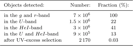
The number of all selected stellar sources in theg- and r-bands from these 211 square degrees is 7×106_{(on average}

3.3×104 per square degree). The number of objects that have aU-band detection is 1.5×106 _{(22%), the number of}

objects with a Heiλ5875 band detection is 3×106 (41%)

and the number of objects with both a U- and Heiλ5875

band detection is 9 ×105 (13%). There are 6.3 × 105 sources that have a U-band detection but no Heiλ5875

detection. These sources are clearly visible in the He_iλ5875

images but have morphology class 0 (‘noise-like’), which we allowed in the U- and Heiλ5875 bands. As a final check

the UVEX_{finder charts of sources that pass the selection} algorithm were eye-balled. Blended objects, sources with noise, double sources and sources close to a bright star are removed. The eye-balling was done in a conservative way: sources with a small artefact which still might be okay were also removed. Only 3% of the UV-excess candidates was removed in the eye-balling. Five percent of the sources was removed because of duplicate entries in the catalogue due to field overlap. This is consistent with the overlap between direct fields and overlap fields (Gonz´alez-Solares et al., 2008). The total number of unique sources that pass the UV-excess selection is 2 170 UV-excess sources and 9 872 additional ‘subdwarfs’. The numbers in this paragraph are summarized in Table 1.

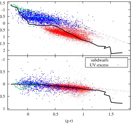
All UV-excess candidates and ‘subdwarf’ sources are plotted in the colour-colour and colour-magnitude diagrams of Figs. 6 and 7. A global photometric calibration is not applied to the UVEXdata yet, so the magnitudes and colours of the UV-excess sources plotted in Figs. 6 and 7 might show a small scatter. The synthetic colours in the colour-colour diagrams are different from the simulated colours in G09 since they include the effect of theU-band filter red leak (see Appendix B). In the colour-magnitude diagrams and in the (U −g) vs. (g−r) colour-colour diagram it can be seen that the UV-excess candidates and the subdwarf sample separate.

Of the objects in the UV-excess catalogue 98% is selected ing vs. (g−r), 66% is selected ing vs. (U −g), 82% is selected in g vs. (g−r) more than 0.4 magnitude from the blue edge, 63% is selected ing vs. (U −g) more than 0.4 magnitude from the blue edge, 44% is selected in both colour-magnitude diagrams more than 0.4 magnitude from the blue edge, and 63% is selected in the (U −g) vs. (g−r) colour-colour diagram. Of the UV-excess candidates 34% is selected 0.4 magnitude from the blue edge ing vs. (g−r) but completely not ingvs. (U−g) and 2% is selected 0.4 magnitude from the blue edge in g vs. (U −g) but completely not ing vs. (g−r). Without theU-band filter 16% of the sources would not be selected in the UV-excess catalogue.

The number of UV-excess objects that have a ‘stellar’ or ‘probably stellar’ U-band detection is 1546 (71.2%), the number of objects with a ‘stellar’ or ‘probably stellar’ Heiλ5875 band detection is 667 (30.7%) and the number

of objects with both a ‘stellar’ or ‘probably stellar’U-band and Heiλ5875 band detection is 513 (23.6%).

-1.5

-1

-0.5

0

0.5

1

1.5

2

(U-g)

-1

-0.5

0

0.5

1

0

0.5

1

1.5

(HeI-r)

(g-r)

subdwarfs

UV-excess

Figure 6.UVEX colour-colour diagrams with all UV-excess candidates (blue) and ’subdwarfs’ (red) selected from the first 211 square degrees of UVEX data. Overplotted are the new simulated unreddened main-sequence (solid black) and the O5V- and supergiant reddening lines (dashed black). These new synthetic colours are different from the colours in G09 since they include the effect of the

13

14

15

16

17

18

19

20

21

22

-1.5

-1

-0.5

0

0.5

1

1.5

g

(U-g)

0

0.5

1

1.5

(g-r)

subdwarfs

UV-excess

Figure 7.UVEX colour-magnitude diagrams with all UV-excess candidates (blue) and ’subdwarfs’ (red) selected from the first 211 square degrees of UVEX data. Since a global photometric calibration was not applied yet the colours plotted here might be scattered a bit.

the purple sample 100% is selected in the (U−g) vs. (g−r) colour-colour diagram, 6% is also selected in gvs. (U−g) more than 0.4 magnitude from the blue edge and 0% is also selected ingvs. (g−r) more than 0.4 magnitude from the blue edge. These sources more than 0.4 magnitude from the blue edge are not in the UV-excess catalogue. Of the purple sources 87% is selected only in the (U−g) vs. (g−r) colour-colour diagram but not at all in a colour-magnitude diagram.

3.1 The properties of the selected UV-excess catalogue

The complete UV-excess catalogue and the two additional ‘subdwarf’ and ‘purple’ samples can be obtained from

Table 1.All (probably) stellar sources from 211 sq.deg.

Objects detected: Number: Fraction (%):

in thegandr-band 7×106 100 in theU-band 1.5×106 22 in theHeI-band 3×₁₀6 ₄₁ in theUandHeI-band 9×₁₀5 ₁₃ after UV-excess selection 2 170 0.03

the UVEXwebsite2 _{or via VizieR}3_{. The columns of the}

catalogue and the different selection labels are explained in

2 _{http://www.uvexsurvey.org}

10

100

No of sources/sq.deg.

Stellar objects (x 1000)

UV-excess

0.1

-4

-2

0

2

4

No of UV-excess/Stellar (x 1e-3)

b (degrees)

UV-excess

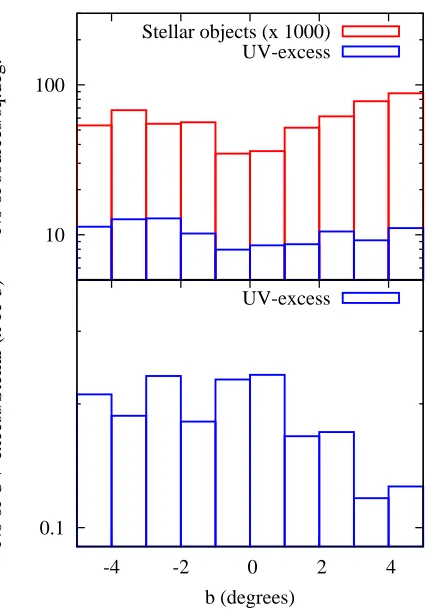
Figure 8.Distribution of stellar sources and UV-excess sources over Galactic latitude (upper graph). The y-axis (in logscale) shows the number of stellar sources and UV-excess candidates per square degree for the associated Galactic latitude bin. The bottom graph shows the ratio of UV-excess candidates and stel-lar sources distributed over Galactic latitude.

Appendix A.

Both the stellar sources and UV-excess candidates se-lected from the 211 square degrees ofUVEXdata are non-uniformly distributed over Galactic latitude and longitude. Fig. 8 shows the distributions of all stellar objects and UV-excess objects over Galactic latitude. The surface density of all stellar sources in ther- and g-bands shows a minimum centred on the Galactic equator. The distribution of the UV-excess sources is not directly straightforward and depends on Galactic latitude.

4 SOURCE CLASSIFICATION AND CROSS-MATCHES WITH OTHER CATALOGUES

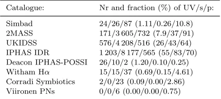
In Sect. 3 we have selected the UV-excess catalogue and two additional samples: a ‘subdwarf’ sample and a ‘purple’ sample. Despite these names each class is expected to consist of a mix of populations. For instance the UV-excess sample will contain white dwarfs, Cataclysmic Variables, AM CVn stars and central stars of planetary nebulae. We have therefore cross-correlated our samples with known source catalogues, the results of which are shown in Figs. 9

to 12 and summarized in Table 2. Spectroscopic follow-up has also been obtained and will be presented in Verbeek et al., 2011b (in prep.).

4.1 Matches with the Simbad database

There are 24 matches (only∼1% of all UV-excess sources) between the UV-excess catalogue and known sources in Simbad, using a matching radius of 10 arcsec. These matches are plotted with theirUVEX_{colours and Simbad} classifications in the (U−g) vs. (g−r) and (HeI−r) vs. (g−r) colour-colour and g vs. (g−r) colour-magnitude diagrams of Fig. 9. The UV-excess candidates that are found in Simbad include 2 planetary nebulae, 3 Cataclysmic Variables, 1 DA white dwarf, 2 high proper motion sources, 2 X-ray sources, 1 emission line star, 10 UV sources, 1 IR source and 2 seemingly normal stars.

Additionally there are 26 known objects from the subd-warf sample in Simbad: 1 planetary nebula, 1 X-ray source, 1 UV source, 1 Mira star, 1 Carbon star, 2 IR sources, 1 radio source, 3 galaxies, 2 variable stars and 13 seemingly normal stars. There are 87 objects from the purple sample in Simbad: 2 X-ray sources, 4 T Tauri stars, 6 Mira stars, 5 Carbon stars, 12 emission line stars, 44 IR sources, 1 radio source, 2 galaxies, 3 variable stars and 8 seemingly normal stars. The fact that three planetary nebulae are found in Simbad shows that in the UVEX_{data the central star is} visible.

4.2 IPHAS_{: The Deacon, Corradi, Viironen and}

Witham catalogues

The INT/WFC Photometric Hα Survey of the Northern Galactic Plane (IPHAS) (Drew et al., 2005) images the same survey area as UVEX_{with the same telescope and} camera set-up using ther,iandHαfilters. The astrometric precision of IPHAS_{is better than 0.1 arcsec (Gonz´} alez-Solares et al., 2008) and on the same frame as UVEX. TheIPHAS_{initial data release (IDR) covers approximately} 89 percent of the total survey area. The result of the cross-matching with a match radius of 1.0 arcsec between our UV-excess catalogue and the IPHAS_{IDR is displayed} in the (r−Hα) vs. (r−i) colour-colour diagram of Fig. 10. Although the match radius of 1.0 arsec is much larger than the astrometric precision of both surveys, it makes sure that all matches are found while it is still too small for mismatches (see Gonz´alez-Solares et al., 2008, Fig. 6). Close neighbours and ambiguities in the UV-excess catalogue were already removed in the eye-balling process.

12

14

16

18

20

g

EM

C

IR

-0.4

-0.2

0

0.2

0.4

0.6

(HeI-r)

Rad

X

PM

CV

PN

TT

-1.5

-1

-0.5

0

0.5

1

-0.5

0

0.5

1

1.5

2

(U-g)

(g-r)

Mi

*

Var

WD

UV

G

Figure 9.Matches between the UV-excess catalogue and Sim-bad plotted in theUVEXcolour-colour and colour-magnitude di-agrams. The black solid lines are the simulated colours of unred-dened main-sequence stars, the dashed lines are the unredunred-dened DA and DB white dwarf tracks (cyan and green) and the O5V-and supergiant reddening line (black dashed). A part of the matches between the additional subdwarf and purple samples and Simbad are also plotted. The legend continues in the three sub-panels. The Simbad object types plotted here are: Emission-line star (EM), Carbon star (C), Infra-Red source (IR), Radio-source (Rad), X-ray Radio-source (X), High proper-motion star (PM), Cataclysmic Variable star (CV), Planetary Nebula (PN), T Tau-type star (TT), Mira-Tau-type star (Mi), star (*), Variable star (Var), White dwarf (WD), UV-emission source (UV) and Galaxy (G).

Additionally 8177 objects of the subdwarf sample and 565 objects of the purple sample have a match in the IPHAS_{IDR. The subdwarfs are at the position of slightly} reddened (E(B−V)<1) A-type stars in the (r−Hα) vs. (r−i) colour-colour diagram of Fig. 10. A small fraction of the purples is saturated in the i-bandIPHASIDR data (∼ 20% of the purples that do not have an IPHASIDR

-0.5 0 0.5 1 1.5

-0.5 0 0.5 1 1.5

(r-H

α

)

(r-i)

Figure 10.All matches between the UV-excess catalogue (blue dots), the two additional subdwarf (red) and purple (black) sam-ples and the IPHAS Initial Data Release plotted in the IPHAS (r-Hα) vs. (r−_i) colour-colour diagram. Overplotted are the sim-ulated main-sequences withE(B−_V) = 0 and _E(_B−_V) = 2 (black solid lines) and the unreddened Koester DA white dwarf track (cyan).

match), an other fraction is blended in theIPHAS_images. In the (r−Hα) vs. (r−i) colour-colour diagram it becomes clear that the purple sample separates out in several sub-samples: one or more is located below the position of the K- and M-dwarfs of the simulated unreddened main-sequence colours at (r−Hα)∼0.4 and (r−i)∼1, a second population is located below the position of the late type stars at reddeningE(B−V)∼2 around (r−Hα)∼1 and (r−i)∼3. There is possibly a third population of Hα emission line objects.

FromIPHASseveral catalogues were selected for high-proper motion objects, Hα emission line stars, Symbiotic stars and planetary nebulae candidates. The result of the cross-match between these catalogues and the UV-excess catalogue is shown in the next subsections.

4.2.1 High-proper motion systems: IPHAS-POSS1 proper motion stars

The IPHAS-POSS1 Proper Motion catalogue (Deacon et al., 2009) is constructed from POSS-I Schmidt plate data taken in the 1950s and 1400 square degrees of IPHAS_Galactic Plane Survey data as a second epoch. This proper motion catalogue has roughly a fifty years baseline and contains populations such as main-sequence stars, white dwarfs, sub-dwarfs and Cataclysmic Variables. The catalogue contains ∼ 105 _{objects with proper motions smaller than 150}

0

1

2

3

(r-H

α

)

Deacon

Witham

Corradi

Viironen

19

20

21

22

23

-0.5

0

0.5

1

1.5

2

2.5

H

(r-i)

UV-excess

subdwarf

purple

Figure 11. IPHAS (r−_Hα) vs. (_r−_i) colour-colour diagram (upper graph) with the matches between the UV-excess cata-logue, the subdwarf and purple samples and the IPHAS-POSS1 catalogue (blue open triangles), Witham Hα emitters (red cir-cles), Corradi symbiotic candidates (black triangle) and Viironen planetary nebulae (green diamonds). The black solid lines are the main-sequence at E(B-V)=0 and E(B-V)=2, the dashed line is the unreddened synthetic Koester DA white dwarf track. The bottom graph shows all objects of the IPHAS-POSS1 proper motion cat-alogue (green dots) in the reduced proper motion diagram and the matches between the UV-excess catalogue and the IPHAS-POSS1 catalogue overplotted. The blue, red and black points are respectively matches with the UV-excess catalogue, subdwarf sample and purple sample. There is one additional purple source at (r−i)=3.4, (r−Hα)=0.9,H_r=19.

the reduced proper motion (Hr) diagram andIPHAS

colour-colour diagram of Fig. 11 together with all the objects in the Deacon IPHAS-POSS1 catalogue. Here reduced proper mo-tion is defined asHr=r+ 5log(µ) + 5, whereris ther-band

magnitude andµis the proper motion in arcseconds per year (see Deacon et al., 2009). The majority of the proper mo-tion UV-excess sources overlaps the white dwarf populamo-tion around (r−i) ∼ 0. In the (r−Hα) vs. (r−i) colour-colour diagram the UV-excess sources mainly overlap with the simulated unreddened white dwarfs track. Also in the UVEX_{colour-colour diagrams of Fig. 12 the matches with} the IPHAS-POSS1 catalogue overlap with simulated white dwarfs tracks. Additionally there is a match for 9 objects from the subdwarf sample and 2 objects from the purple sample.

4.2.2 Hα-emission line systems: Witham IPHAS Hα emission-line objects

The Witham catalogue of Hαemission-line objects (Witham et al., 2008) is extracted from ∼80 percent of the IPHASGalactic Plane Survey area data. This catalogue, se-lected from the (r−Hα) vs. (r−i) colour-colour diagram, contains 4853 point sources clearly showing Hα-excess. Spec-troscopic follow-up of∼300 candidates shows that more than 95 percent are indeed true Hα emitters such as early-type emission-line stars, active late-type stars, interacting bina-ries, young stellar objects and compact nebulae (see Wesson et al., 2008, Viironen et al., 2009). When the UV-excess cat-alogue is cross-matched with the Witham catcat-alogue there is a match within a radius of 1.0 arcsec for 15 UV-excess candidates and additionally there is a match for 15 objects in the subdwarf sample and 37 objects in the purple sample. These matches are plotted in Figs. 11 and 12.

4.2.3 Symbiotic stars: Corradi IPHAS symbiotic catalogue

Symbiotic stars (see e.g. Corradi et al., 2008 and 2010) are interacting binaries composed of a hot white dwarf, accret-ing from a cool giant companion through a wind or through Roche lobe overflow. Two types “Stellar” (S) and “Dusty” (D) exist with orbital periods between 1-16 years, and more than 20 years, respectively. The number of known systems in our Galaxy, where 80 percent is S-type, is roughly 200 including 26 suspected candidates, but the size of the total symbiotic population in the Milky Way is still poorly known (Belczy´nski et al., 2000). The IPHAS_{symbiotic catalogue} (Corradi et al., 2008) was extracted from IPHAS_Galactic Plane Survey data. Cross correlating theIPHASsymbiotic catalogue (Corradi et al., 2008) with the UV-excess cata-logue results in a match for 2 sources within a radius of 1.0 arcsec. Additionally there is a match for 23 purple sources. These matches are also in the Witham Hα emission line star catalogue. This large fraction of purple matches is due to the position of the symbiotic stars in theUVEX colour-colour diagrams, see Fig. 12. In the (HeI−r) vs. (g−r) colour-colour diagram the symbiotic candidate matches are to the right of the characteristic “hook” of the simulated unreddened main-sequence colours. Note that a fairly large fraction of the sources in the IPHASsymbiotic catalogue (Corradi et al., 2008) are likely to be young stellar ob-jects. For most of the symbiotic candidate matches the avail-able spectroscopic data were checked. The majority of the UVEX_{symbiotic candidate matches turn out to be classical}

T Tauri stars (Verbeek et al., 2011b, in prep.) while none of them is a known symbiotic star, and they are found in regions of the sky close to other Hα emitters. When the UVEX_{colours of these matches are compared with} simu-lated symbiotic colours the colours of the symbiotic can-didate matches are too blue. Therefore, these matches are not good symbiotic star candidates as symbiotic stars in the Galactic Plane are generally redder.

4.2.4 Planetary Nebulae: Viironen IPHAS Planetary Nebulae

-1.5 -1 -0.5 0 0.5 1 1.5 (U-g) Witham Deacon Corradi Viironen -0.2 -0.1 0 0.1 0.2 0.3 0.4 0.5 0.6 0.7

0 0.5 1 1.5 2

(HeI-r)

(g-r)

Figure 12.Result of the cross-matching between the UV-excess catalogue, the subdwarf and purple samples and the IPHAS Hαemission line objects (Witham), IPHAS-POSS1 high proper motion stars (Deacon), IPHAS symbiotic candidates (Corradi) and IPHAS planetary nebula candidates (Viironen), overplotted on the simulated unreddened main-sequence (solid black line) and the unreddened DA and DB white dwarf tracks (cyan and green lines). The dashed lines are the O5V-reddening line (upper graph) and the supergiant reddening line (bottom graph). There is one additional purple source at (g−_r)=3.02, (_U−_g)=2.22, (r−_HeI)=1.19.

a white dwarf, have been found in the Milky Way so far while population syntheses predicts a larger population (4.6±1.3 Galactic PN with radii < 0.9pc, Moe et al., 2006). Ex-tinction makes it difficult to observe planetary nebulae in the direction of the Galactic Plane. The Viironen plane-tary nebula catalogue (Viironen et al., 2009) contains 781 planetary nebula candidates selected from theIPHASdata. The list includes very young and proto-planetary nebulae, normal planetary nebulae and other non-planetary nebula emission line objects. Cross-correlating the Viironen cata-logue with the UV-excess catacata-logue results in 0 matches within 1.0 arcsec. Only from the purple sample 6 objects have a match with the Viironen catalogue. These planetary candidate matches are in the same regime as the symbi-otic candidates matches. Their location in theIPHAS_and UVEXcolour-colour diagrams is shown in Figs. 11 and 12. None of the matches is a known planetary nebula, and due to the blueUVEXcolour of these matches they are not good planetary nebulae candidates.

Table 2.Summary of the cross-matching.

Catalogue: Nr and fraction (%) of UV/s/p:

Simbad 24/26/87 (1.11/0.26/10.8) 2MASS 171/3 605/732 (7.9/37/91) UKIDSS 576/4 208/516 (26/43/64) IPHAS IDR 1 203/8 177/565 (55/83/70) Deacon IPHAS-POSSI 26/10/2 (1.20/0.10/0.25) Witham Hα 15/15/37 (0.69/0.15/4.61) Corradi Symbiotics 2/0/23 (0.09/0.00/2.86) Viironen PNs 0/0/6 (0.00/0.00/0.75)

4.3 The Two-Micron All-Sky Survey

The selected UV-excess sample is cross-matched with the Two-Micron All-Sky Survey (2MASS) data (Cutri et al., 2003). Of the UV-excess candidates 171 objects can be found in 2MASS within a radius of 1.0 arcsec. Additionally there is a match in 2MASS for 3605 subdwarfs and 732 purple sources. This shows the good match ofUVEXwith 2MASS, in particular for the redder sources. The cross-match between the UV-excess catalogue, subdwarf and puple samples and 2MASS will be further discussed in Verbeek et al., 2011c (in prep.).

4.4 The UKIRT InfraRed Deep Sky Surveys Finally the UV-excess catalogue is cross-matched with the the UKIDSS (UKIRT InfraRed Deep Sky Surveys) Galactic Plane Survey (Lucas et al., 2008). This survey images the Northern Galactic plane in the same Galactic latitude range as UVEX in the filtersJ,HandK. There is a match for 576 UV-excess candidates within a radius of 1.0 arcsec in one of the filters. Of these UV-excess candidates 219 sources have a matches in all three filters. Additionally there is a match for 4208 subdwarfs and 506 purples. The cross-match between our samples and the UKIDSS GPS will also be further discussed in Verbeek et al., 2011c (in prep.).

5 DISCUSSION AND CONCLUSIONS

We present the first catalogue of UV-excess sources se-lected from a total of 7×106 _{stars in 211 square degrees}

of UVEXdata. This catalogue contains 2 170 unique UV-excess candidates with magnitudes between 14< g <22.5. With the selection technique presented in Sect. 2 we select on average ∼11 UV-excess candidates per square degree. Cross-matching with other catalogues shows that the UV-excess catalogue consist of a mix of populations with only a small fraction that has been identified before.

5.1 Completeness and reliability of the UV-excess catalogue

-1

0

1

2

3

0

0.5

1

1.5

2

2.5

(U-g)

(g-r)

UVEX 4294

Figure 13.(U−_g) vs. (_g−_r) colour-colour diagram of field UVEX 4294. Data shown are all stellar and probably stellar detections (red dots) of field UVEX 4294 (l=43.88, b=4.67). The lines show the line fitted to the main locus (central line) and the 3σ wide selection box. The blue, red and black data points are respectively the UV-excess, subdwarf and purple candidates selected from this field. The 4 magenta data points show subdwarfs selected in the blue corner of the colour-colour diagram outside the selection box but less than 0.4 magnitude from the blue edge in the colour-magnitude diagrams. The black solid lines are the simulated colours of main-sequence stars with E(B-V)=0 and E(B-V)=2, the dashed lines are the unreddened DA white dwarf tracks (cyan) and the O5V-reddening line (black dashed).

0.1 0.2 0.3 0.4 0.5 0.6 0.7 0.8 0.9 1

(g-r)

g

-0.5 0 0.5 1 1.5

14

16

18

20

22

Figure 14.Probability that a source will be picked-up by the selection algorithm of Sect.2 depending on the position of the source in thegvs. (g−_r) colour-magnitude diagram.

main-sequence may still be selected when they are slightly scattered. In the colour-magnitude diagrams (see Figs. 1 and 2) the edge of the selection line (left ‘ragged’ solid line) may become rather ‘jumpy’ when only a small number of main-sequence objects is detected, leading to a loss of objects or the inclusion of too many objects at the brighter or fainter ends. For example in theg vs. (U−g) colour-magnitude diagram of Fig. 1 there is one object at g∼21 not selected as UV-excess candidate due to the blue edge of the last bin. The number of UV-excess candidates in the catalogue brighter thang <16 is 23. Fig. 15 shows the magnitude distributions of the UV-excess sources. The number of selected UV-excess sources increases for fainter magnitudes. The probability that a source with a particular (g−r) colour and g-band magnitude will be picked-up in our 211 square degrees is given in Fig. 14. For a given (g−r) colour the probability for faint sources to be selected is larger than for bright objects.

0

1

2

3

4

r

g

UV-excess

subdwarfs

0

1

2

3

4

5

14

16

18

20

22

No of UV-excess candidates / No of Stellar sources

magnitude

U

14

16

18

20

22

magnitude

HeI

Figure 15. r-, g-, U-, and HeI-band magnitude distributions of the UV-excess candidates (solid/blue) and the ‘subdwarf’ sample (dot-dashed/red). In the histograms the number of UV-excess candidates and subdwarfs is devided by the number of stellar sources in the magnitude bin and normalized to one by the total number of UV-excess, subdwarf and stellar sources.

Fig. 13. In field UVEX_{4294 there are 19 sources selected} in the blue corner of the (U −g) vs. (g−r) colour-colour diagram outside the selection box. Four of these sources (magenta in Fig. 13) are less than 0.4 magnitude from the blue edge in the colour-magnitude diagrams and are in the ‘subdwarf’ sample. Three of these ‘subdwarf’ sources are probably early-type stars since they are too close to the main locus, the fourth ‘subdwarf’ is near the location of the UV-excess sources. The 15 UV-excess candidates in Fig. 13 are more than 0.4 magnitude from the blue edge in the colour-magnitude diagrams and are on top of the unreddened white dwarf track. In very sparse fields without blue or UV-excess sources the fit of the straight line in the (U−g) vs. (g−r) colour-colour diagram may be completely wrong, but this is no problem since these fields will not contribute new UV-excess objects to our catalogue anyway.

Guaranteeing that every object in the UV-excess catalogue is indeed a real UV-excess source is impossi-ble, although first preliminary spectroscopic follow-up observations (Verbeek et al., 2011b, in prep.) show that at least 80% of the UV-excess candidates are indeed genuine UV-excess sources such as white dwarfs and white dwarf binaries. As can be seen in Fig. 5 the tails of the

to use a conservative selection method.

5.2 The two additional subdwarf and purple samples

Two additional sub-samples of 9 872 objects labelled as ‘subdwarf’ candidates and 803 objects labelled as ‘pur-ple’ sources are selected from the 211 square degrees of UVEX_{data. The subdwarf sample is slightly bluer than} the main-sequence and contains a mix of metal-poor stars and lightly reddened main-sequence stars. Fig. 13 shows the colour-colour diagram of fieldUVEX_{4294 where most} ‘sub-dwarf’ sources, selected in thegvs. (g−r) colour-magnitude diagram, overlap with the earliest main-sequence stars in this field. Fig. 15 shows the number of subdwarfs divided by the number of stellar sources per magnitude bin. There is a bump in theg-band andU-band magnitude distributions for the bright subdwarfs. The bright subdwarfs are selected in the g vs. (g−r) colour-magnitude diagram and in the g vs. (U −g) colour-magnitude diagram but not in the (U−g) vs. (g−r) colour-colour diagram. This is because the first bins of the blue edge in Fig. 1 are usually larger, while the sources of the main locus change over (g−r) or (U −g) in these first bins. In field UVEX4294 there are 9 sources at the purple side more than 3 σ outside the selection box. Only the 4 purple sources that are above the O5V-reddening line are selected in the ‘purple’ sample since the other sources might be scattered reddened main-sequence stars. Only when there are large magnitude offsets in (g−r) or (U −g) this demand might cause problems. Fields with obvious magnitude offsets in (g−r), (U −g) or in (HeI −r) were removed in Sect. 3. In the (U−g) vs. (g−r) colour-colour diagram it is not possible to use the reddening vector to fit a straight line to the main locus since each field will consist of a mix of popula-tions at different distances subjected to different reddenings.

The cross-matching with other catalogues and databases (Deacon, Corradi, Viironen, Witham, 2MASS, UKIDSS and Simbad) shows that ∼1 percent of the UV-excess sources were previously known objects and∼77 percent were previously detected by IPHAS_{. The vast} majority of objects are not classified yet, soUVEX_uncovers a large new sample of white dwarfs, subdwarfs, Cataclysmic Variables, symbiotic stars, planetary nebulae and other post-common-envelope objects.

ACKNOWLEDGEMENT

This paper makes use of data collected at the Isaac Newton Telescope, operated on the island of La Palma by the Isaac Newton Group in the Spanish Observatorio del Roque de los Muchachos of the Inst´ıtuto de Astrof´ısica de Canarias. The observations were processed by the Cambridge Astron-omy Survey Unit (CASU) at the Institute of AstronAstron-omy, University of Cambridge. This work is based in part on data obtained as part of the UKIRT Infrared Deep Sky Survey (UKIDSS). We acknowledge the use of data products from Two-Micron All-Sky Survey (2MASS), which is a joint

project of the University of Massachusetts and the Infrared Processing and AnalysisCenter/California Institute of Technology (funded by the National Aeronautics and Space Administration and National Science Foundation of the USA). This research has made use of the Simbad database and the VizieR catalogue access tool, operated at CDS, Strasbourg, France. KV is supported by a NWO-EW grant 614.000.601 to PJG. The authors would like to thank Detlev Koester and Pierre Bergeron for making available their white dwarf models on which a significant part of the colour simulations in this paper are based. The authors want to thank allUVEX_{observers for going to La Palma.}

REFERENCES

Belczynski K., Mikolajewska J., Munari U., et al.,2000 A&A 146, 407

Bergeron P., Wesemael F. & Beauchamp A., 1995, PASP 107, 1047

Cardelli J.A., Clayton G.C. & Mathis J.S., 1989, ApJ 345, 245

Corradi R. L. M., Rodriguez-Flores E. R., Mampaso A., et al., 2008 yCat 34800409

Corradi R. L. M., Valentini M., Munari U., Drew J. E., et al., 2010 A&A 509, 41

Cutri R. M., Skrutskie M. F., van Dyk S. et al., 2003, yCat 2246, 0

Deacon N. R., Groot P. J., Drew J. E., et al., 2009, MN-RAS.397, 1685

Drew J., Greimel R., Irwin M., et al., 2005, MNRAS 362, 753 (D05)

Drew J., et al., 2008, MNRAS 386, 1761

Gonz´alez-Solares E.A., Walton N.A., Greimel R., Drew, J.E., et al., 2008, MNRAS 388, 89

Groot P.J., Verbeek K., Greimel R., et al., 2009, MNRAS 399, 323G

Johnson H. L., Knuckles, C. F., 1955, ApJ 122, 209 Koester D., et al., 2001, A&A, 378, 556

Lucas P. W., et al, 2008, 2008MNRAS.391..136L Moe M., De Marco O., 2006, ApJ 650, 916

Nelemans G., Yungelson L & Portegies Zwart, 2004, MN-RAS 349, 181

Pretorius, M. L., Knigge, C., Kolb, U., 2007, MNRAS 374, 1495

Pickles A.J., 1998, PASP 110, 863

Sale S., Drew J., Unruh Y., et al., 2009, MNRAS 392, 497 Schlegel D.J., Finkbeiner D.P. & Davis, M., 1998, ApJ 500,

525

Viironen K., Greimel R., Corradi R. L. M., et al., 2009, A&A 504, 291

Wesson R., Barlow M., Corradi R., et al., 2008, ApJ 688, L21

APPENDIX A: CATALOGUE OF UV-EXCESS CANDIDATES

The complete UV-excess catalogue, and the two additional ‘subdwarf’ and ‘purple’ samples, selected from the first 211 square degrees of UVEXdata can be obtained at the UVEX_website4 _{or via VizieR}5_{. The UV-excess catalogue,} the ‘subdwarf’ and ‘purple’ samples contain 50 columns:

1–6: RA and dec. 7:UVEX_field.

8–19: rav, ∆r, morp.class r, gav, ∆g, morp.class g, Uav,

∆U, morp.classU,Heav, ∆He, morp.classHe.

20:UVEX_{selection flag.}

21: (U−g)BlueEdge- (U−g)source - 2σ(U−g); the difference

in (U −g) between source and the blue edge in theg vs. (U−g) colour-magnitude diagram, inclusive the photomet-ric error of the source.

22: (g−r)BlueEdge- (g−r)source- 2σ(g−r); the difference in

(g−r) between source and the blue edge in thegvs. (g−r) colour-magnitude diagram, inclusive the photometric error of the source.

23–34: Original magnitudes, magnitude errors and mor-phology classes from the direct field: r, ∆r, morp.class r, g, ∆g, morp.class g, U, ∆U, morp.class U, He, ∆He, morp.classHe.

35–46: Original magnitudes, magnitude errors and mor-phology classes from offset field:r, ∆r, morp.classr,g, ∆g, morp.class g, U, ∆U, morp.class U,He, ∆He, morp.class He.

47–50: Average rav.f ield, gav.f ield, Uav.f ield, HeIav.f ield

magnitude of the total field.

– Columns 8, 11, 14 and 17 contain averaged magni-tudes (rav, gav,Uav and Heav) over direct field and offset

field. These magnitudes, corrected for magnitude shifts between field and offset field, are calculated in a few steps, e.g. forrav:

i) first (rdirect−rof f set) is calculated for each coordinate

match between a field and offset field,

ii) from this (rdirect−rof f set) distribution the first 25%

and last 25% is removed,

iii) from the central 50% the mean magnitude shift (rshif t)

between direct field and offset field is calculated,

iv) the magnitudes of the offset field are corrected for magnitude shifts byrof f setN EW=rof f set− |rshif t|,

v) per source the magnitude difference of direct field and offset field is checked: do the magnitudes match within the error bars? Here an extra 0.05 mag is taken into account to avoid that too much sources are removed.

vi) the averaged magnitude rav is now simply calculated

by:rav=(rdirect+rof f setN EW)/2.

– Columns 10, 13, 16 and 19 are “averaged” morphol-ogy class flags of the direct field and offset field: the best flag of the two. The possible morphology classes are: -1 (stellar), -2 (probably stellar) and 0 (noise-like).

– Column 20 is the UVEX_{selection flag (1, 2, 4, 32,}

4 _{http://www.uvexsurvey.org} 5 _{http://vizier.u-strasbg.fr/viz-bin/VizieR} 0 0.02 0.04 0.06 0.08 0.1

2000 3000 4000 5000 6000 7000 8000 9000

Throughput (%)

Wavelength (Angstrom) INT/WFC #204 RGO U

Figure B1.Throughput of the INT/WFC RGO U-band filter used for UVEX with the red leak near 7050˚A.

64, 512, 1024 or combinations) and gives information about how the source was selected:

1) outlier on the blue side of the main-sequence in the (U−g) vs. (g−r) colour-colour diagram.

2) outlier on the blue side of the main-sequence in thegvs. (U−g) colour-magnitude diagram.

4) outlier on the blue side of the main-sequence in thegvs. (g−r) colour magnitude diagram.

32) outlier on the purple side of the main-sequence in the (U−g) vs. (g−r) colour-colour diagram.

64) outlier on the non-purple side of the main-sequence in the (U−g) vs. (g−r) colour-colour diagram.

512) outlier on the blue side of the main-seq in the g vs. (U −g) colour-magnitude diagram that lies more than 0.4 mag away from the main-sequence blue edge.

1024) outlier on the blue side of the main-seq in theg vs. (g−r) colour-magnitude diagram that lies more than 0.4 mag away from the main-sequence blue edge.

APPENDIX B: SYNTHETIC COLOURS WITH THE EFFECT OF THEU-BAND FILTER “RED LEAK”.

-2

0

2

4

6

8

-1 0 1 2 3 4 5

(U-g)

(g-r) 0.0

2.0

4.0 O5V reddening line

M0III reddening line

Figure B2.The synthetic colours of main-sequence stars, giants and super giants including the effect of theU-band filter red leak plotted in the (U−_g) vs. (_g−_r) colour-colour diagram. The colour-colour diagram without the effect of theU-band red leak was already shown in G09 (Fig.6). In this graph the black lines are the old G09 colours, the overplotted lines are the new syn-thetic colours of main-sequence stars (thick red), giants (blue) and super giants (thin red) for E(B–V)=0.0, 2.0 and 4.0 using the reddening law of Cardelli et al. (1989). The upper and lower envelope curves (dashed) are the old O5V-reddening curve and the M0III-reddening curve of G09. Late M-giants from M7III to M10III, not shown in G09, were add.

Table B1.UVEXcolour indices (U−_g), (_g−_r), (_HeI−_r) for Pickles main-sequence stars including reddening.

Table B2.UVEXcolour indices (U−_g), (_g−_r), (_HeI−_r) for Pickles Giants including reddening.

Spec. E(B−_V)=0.0 _E(_B−_V)=1.0 _E(_B−_V)=2.0 _E(_B−_V)=3.0 _E(_B−_V)=4.0 type U−_{g g}−_{r Hei}−_{r U}−_{g g}−_{r Hei}−_{r U}−_{g g}−_{r Hei}−_{r U}−_{g g}−_{r Hei}−_{r U}−_{g g}−_{r Hei}−_r O8III –1.341 –0.259 0.001 –0.152 0.696 0.143 1.122 1.571 0.320 2.450 2.383 0.532 3.689 3.154 0.777 B1-2III –1.133 –0.215 0.016 0.053 0.733 0.160 1.322 1.603 0.340 2.642 2.412 0.554 3.841 3.181 0.801 B3III –0.820 –0.185 0.032 0.362 0.759 0.179 1.625 1.627 0.361 2.931 2.435 0.578 4.057 3.204 0.828 B5III –0.594 –0.132 0.010 0.577 0.812 0.158 1.828 1.679 0.341 3.114 2.487 0.559 4.175 3.256 0.810 B9III –0.143 –0.045 –0.002 0.999 0.895 0.147 2.220 1.757 0.330 3.461 2.561 0.548 4.385 3.326 0.799 A0III 0.016 0.040 –0.003 1.172 0.968 0.147 2.405 1.821 0.333 3.642 2.618 0.552 4.483 3.377 0.805 A3III 0.168 0.136 –0.008 1.324 1.054 0.145 2.553 1.899 0.334 3.772 2.689 0.556 4.526 3.445 0.812 A5III 0.185 0.172 0.031 1.351 1.088 0.186 2.590 1.932 0.377 3.807 2.722 0.603 4.511 3.480 0.861 A7III 0.230 0.234 0.025 1.398 1.150 0.183 2.638 1.994 0.376 3.849 2.784 0.602 4.511 3.541 0.862 F0III 0.242 0.276 0.038 1.418 1.186 0.198 2.663 2.026 0.393 3.872 2.815 0.622 4.503 3.571 0.883 F2III 0.206 0.437 0.060 1.408 1.337 0.226 2.677 2.169 0.427 3.884 2.952 0.662 4.427 3.704 0.929 F5III 0.241 0.451 0.074 1.446 1.352 0.242 2.715 2.186 0.444 3.915 2.971 0.680 4.424 3.726 0.948 G0III 0.564 0.663 0.106 1.801 1.544 0.281 3.087 2.364 0.490 4.209 3.140 0.732 4.411 3.888 1.006 G5III 0.978 0.822 0.127 2.242 1.686 0.307 3.528 2.493 0.522 4.511 3.261 0.770 4.392 4.007 1.048 G8III 1.136 0.883 0.133 2.396 1.740 0.314 3.669 2.543 0.529 4.583 3.307 0.777 4.365 4.049 1.055 K0III 1.313 0.891 0.162 2.569 1.753 0.346 3.828 2.559 0.564 4.669 3.328 0.815 4.356 4.074 1.096 K1III 1.458 0.972 0.162 2.721 1.826 0.346 3.967 2.628 0.565 4.720 3.393 0.816 4.304 4.137 1.098 K2III 1.589 1.047 0.186 2.842 1.897 0.374 4.066 2.696 0.597 4.736 3.458 0.852 4.248 4.200 1.137 K3III 1.842 1.118 0.191 3.103 1.960 0.380 4.300 2.753 0.603 4.818 3.513 0.859 4.208 4.252 1.145 K4III 2.259 1.303 0.198 3.539 2.123 0.391 4.657 2.900 0.619 4.856 3.647 0.878 4.073 4.377 1.168 K5III 2.364 1.345 0.252 3.621 2.175 0.452 4.681 2.959 0.684 4.770 3.712 0.949 3.944 4.448 1.244 M0III 2.620 1.444 0.327 3.867 2.266 0.532 4.823 3.044 0.770 4.703 3.793 1.041 3.813 4.527 1.341 M1III 2.554 1.449 0.313 3.795 2.272 0.518 4.764 3.050 0.757 4.671 3.800 1.028 3.790 4.533 1.328 M2III 2.675 1.513 0.385 3.913 2.337 0.597 4.803 3.117 0.844 4.578 3.870 1.122 3.663 4.607 1.429 M3III 2.572 1.477 0.470 3.808 2.302 0.688 4.704 3.084 0.939 4.489 3.838 1.221 3.573 4.578 1.532 M4III 2.512 1.507 0.629 3.734 2.335 0.858 4.568 3.120 1.121 4.272 3.880 1.415 3.338 4.625 1.736 M5III 1.930 1.547 0.757 3.161 2.390 0.997 4.115 3.186 1.270 4.001 3.954 1.573 3.112 4.707 1.903 M6III 1.981 1.745 0.944 3.181 2.599 1.203 3.979 3.405 1.494 3.648 4.183 1.814 2.705 4.947 2.159 M7III 1.199 2.029 1.203 2.403 2.905 1.484 3.287 3.724 1.795 3.080 4.512 2.132 2.169 5.283 2.494 M8III 0.403 2.663 1.705 1.655 3.551 2.020 2.541 4.377 2.362 2.291 5.169 2.725 1.378 5.943 3.108 M9III 0.309 1.389 1.344 1.615 2.257 1.629 2.831 3.086 1.946 3.287 3.890 2.289 2.626 4.681 2.656 M10III 0.172 1.149 1.543 1.479 2.031 1.840 2.719 2.872 2.167 3.269 3.689 2.522 2.665 4.492 2.899

Table B3.UVEX_/IPHAS_{colour indices (U}−_g), (_g−_r), (_HeI−_r) for Pickles Supergiants including reddening.

Table B4.UVEX/IPHAScolour indices (U−_g), (_g−_r), (_Hei−_r) (_r−_Hα) and (_r−_i) for log(g)=8.0 Bergeron DA white dwarfs including reddening.

T (K) E(B–V)=0.0 E(B–V)=1.0 E(B–V)=2.0

Table B4., continued

T (K) E(B–V)=3.0 E(B–V)=4.0

Table B5.UVEX/IPHAScolour indices (U−_g), (_g−_r), (_HeI−_r) (_r−_Hα) and (_r−_i) for log(g)=8.0 Koester DA white dwarfs including reddening

T (K) E(B–V)=0.0 E(B–V)=1.0 E(B–V)=2.0

Table B5., continued

T (K) E(B–V)=3.0 E(B–V)=4.0

Table B6.UVEX/IPHAScolour indices (U−_g), (_g−_r), (_HeI−_r) (_r−_Hα) and (_r−_i) for log(g)=8.0 Koester DB white dwarfs including reddening.

T (K) E(B–V)=0.0 E(B–V)=1.0 E(B–V)=2.0

U−_{g g}−_{r Hei}−_{r r}−_{Hα r}−_{i U}−_{g g}−_{r Hei}−_{r r}−_{Hα r}−_{i U}−_{g g}−_{r Hei}−_{r r}−_{Hα r}−_i 10000 –0.753 0.162 0.033 0.172 0.081 0.465 1.083 0.189 0.361 0.781 1.759 1.930 0.380 0.515 1.485 11000 –0.839 0.109 0.031 0.161 0.049 0.376 1.033 0.186 0.351 0.749 1.669 1.883 0.375 0.507 1.453 12000 –0.907 0.067 0.037 0.153 0.023 0.305 0.995 0.190 0.345 0.724 1.597 1.848 0.378 0.502 1.428 13000 –0.955 0.032 0.050 0.146 –0.000 0.256 0.962 0.202 0.339 0.701 1.547 1.816 0.388 0.498 1.406 14000 –0.990 0.001 0.072 0.140 –0.020 0.219 0.933 0.223 0.334 0.681 1.510 1.788 0.408 0.494 1.386 15000 –1.014 –0.024 0.101 0.135 –0.037 0.195 0.908 0.250 0.330 0.665 1.485 1.764 0.435 0.491 1.370 16000 –1.028 –0.045 0.134 0.130 –0.050 0.180 0.888 0.283 0.326 0.652 1.471 1.744 0.466 0.488 1.358 17000 –1.037 –0.063 0.167 0.125 –0.060 0.172 0.870 0.314 0.322 0.643 1.463 1.725 0.497 0.485 1.349 18000 –1.043 –0.078 0.194 0.120 –0.068 0.166 0.855 0.341 0.318 0.635 1.458 1.709 0.522 0.481 1.343 19000 –1.048 –0.091 0.212 0.115 –0.075 0.161 0.841 0.358 0.314 0.629 1.453 1.695 0.539 0.478 1.337 20000 –1.054 –0.103 0.220 0.111 –0.081 0.155 0.830 0.366 0.310 0.624 1.447 1.684 0.546 0.475 1.332 22000 –1.064 –0.117 0.216 0.107 –0.088 0.144 0.816 0.361 0.306 0.617 1.436 1.670 0.541 0.471 1.325 24000 –1.077 –0.128 0.199 0.104 –0.094 0.131 0.807 0.343 0.304 0.611 1.422 1.662 0.523 0.469 1.319 26000 –1.100 –0.142 0.185 0.100 –0.103 0.107 0.793 0.329 0.301 0.602 1.397 1.650 0.508 0.467 1.310 28000 –1.127 –0.156 0.175 0.098 –0.113 0.078 0.781 0.319 0.299 0.592 1.368 1.639 0.497 0.465 1.300 30000 –1.156 –0.169 0.164 0.096 –0.122 0.048 0.770 0.307 0.297 0.583 1.336 1.630 0.485 0.464 1.291 35000 –1.227 –0.196 0.134 0.092 –0.139 –0.025 0.747 0.277 0.294 0.565 1.261 1.611 0.454 0.461 1.274 40000 –1.285 –0.218 0.116 0.088 –0.154 –0.085 0.728 0.258 0.290 0.551 1.199 1.594 0.435 0.459 1.259 50000 –1.418 –0.236 0.038 0.080 –0.180 –0.223 0.717 0.180 0.284 0.524 1.058 1.589 0.355 0.453 1.232

Table B6., continued

T (K) E(B–V)=3.0 E(B–V)=4.0