NBER WORKING PAPER SERIES
RARE DISASTERS AND EXCHANGE RATES Emmanuel Farhi
Xavier Gabaix Working Paper 13805
http://www.nber.org/papers/w13805
NATIONAL BUREAU OF ECONOMIC RESEARCH 1050 Massachusetts Avenue
Cambridge, MA 02138 February 2008
For helpful comments, we thank Andy Atkeson, David Backus, Robert Barro, Daniel Cohen, Alex Edmans, Christian Julliard, Pat and Tim Kehoe, Raj Mehra, Emi Nakamura, Eric van Wincoop, and seminar participants at Boston University, Dartmouth, LBS, LSE, Minneapolis Fed, NBER, New York Fed, NYU, UBC, and the University of Virginia. Gabaix thanks the NSF for support. The views expressed herein are those of the author(s) and do not necessarily reflect the views of the National Bureau of Economic Research.
NBER working papers are circulated for discussion and comment purposes. They have not been peer-reviewed or been subject to the review by the NBER Board of Directors that accompanies official NBER publications.
© 2008 by Emmanuel Farhi and Xavier Gabaix. All rights reserved. Short sections of text, not to exceed two paragraphs, may be quoted without explicit permission provided that full credit, including © notice, is given to the source.
Rare Disasters and Exchange Rates Emmanuel Farhi and Xavier Gabaix NBER Working Paper No. 13805 February 2008
JEL No. E43,E44,F31,G12,G15
ABSTRACT
We propose a new model of exchange rates, which yields a theory of the forward premium puzzle. Our explanation combines two ingredients: the possibility of rare economic disasters, and an asset view of the exchange rate. Our model is frictionless, has complete markets, and works for an arbitrary number of countries. In the model, rare worldwide disasters can occur and affect each country's productivity. Each country's exposure to disaster risk varies over time according to a mean-reverting process. Risky countries command high risk premia: they feature a depreciated exchange rate and a high interest rate. As their risk premium mean reverts, their exchange rate appreciates. Therefore, currencies of high interest rate countries appreciate on average. To make the notion of disaster risk more implementable, we show how options prices might in principle uncover latent disaster risk, and help forecast exchange rate movements. We then extend the framework to incorporate two factors: a disaster risk factor, and a business cycle factor. We calibrate the model and obtain quantitatively realistic values for the volatility of the exchange rate, the forward premium puzzle regression coefficients, and near-random walk exchange rate dynamics. Finally, we solve a model of stock markets across countries, which yields a series of predictions about the joint behavior of exchange rates, bonds, options and stocks across countries. The evidence from the options market appears to be supportive of the model.
Emmanuel Farhi Harvard University Department of Economics Littauer Center Cambridge, MA 02138 and NBER [email protected] Xavier Gabaix
New York University Finance Department Stern School of Business 44 West 4th Street, 9th floor New York, NY 10012 and NBER
1
Introduction
We propose a new model of exchange rates, which yields a theory of exchange rate “excess volatility” and of the forward premium puzzle. We build on the idea proposed by Rietz (1988), Barro (2006) and Weitzman (2007) that the possibility of rare but extreme events is a major determinant of risk premia in asset markets, and develop a tractable framework to study its consequences for international asset prices.
Our model allows us to propose a solution for a major puzzle in international macroeconomics, the failure of uncovered interest rate parity (UIP). According to the UIP equation, the expected depreciation of a currency should be equal to the interest rate differential between that country and the reference region. A regression of exchange rate changes on interest rate differentials should yield a coefficient of 1. However, empirical studies starting with Hansen and Hodrick (1980) and Fama (1984), and recently surveyed by Froot and Thaler (1990), Lewis (1995) and Engel (1996), consistently produce a regression coefficient that is less than1, and often negative. This invalidation of UIP has been termed the forward premium puzzle: currencies with high interest rates tend to appreciate. In other words, currencies with high interest rates feature positive predictable excess re-turns. There are four possible explanations: time-varying risk premia, Peso problems, expectations errors, and illiquid markets1.
Our paper provides a theory of international time-varying risk premia in a complete markets, frictionless and rational framework. In our model, the exchange rate is both a relative price of non-traded and traded goods, and an asset price: it is the net present value of the export sector’s productivity. For this, we develop a “stock view” of the exchange rate. We postulate (to the best of our knowledge, in a novel way), a linear technology by which an initial investment of non-tradable goods yields a stream of future export goods, with stochastic productivity. As a result, the exchange rate is the present value of the country’s future export productivities, discounted using the international pricing kernel. This “stock view” of the exchange rate could be used in other contexts, e.g. with habit formation. In our model, risky countries are those whose productivity will fall by a lot during disasters.
Risky countries command high risk premia: they feature a depreciated exchange rate and a high interest rate. As their risk premium reverts to the mean, their exchange rate appreciates. Therefore, the currencies of high interest rate countries appreciate on average. This provides an explanation for the forward premium puzzle. The model is consistent with a forward premium puzzle, both in sample with and without disasters. Therefore it does not suffer from a Peso problem. The driving force of our result is that the risk premium covaries positively with interest rate. In other words, our theory does not rely on mismeasurement of expectations. We calibrate a version of the model and obtain quantitatively realistic values for the volatility of the exchange rate, the forward premium 1Maynard and Phillips (2001) argue that the forward premium puzzle is the result of misspecification issues. The
Fama (1984) regression assumes short-memory stationarity of the data, but evidence contradicts this. Misspecification arises from long memory in the forward premium (the independent variable), and this may induce a bias away from
puzzle regression coefficients, and near-random walk exchange rate dynamics.
The model is very tractable, and expressions for the exchange rate, interest rate, risk premia, and forward premium puzzle coefficients are obtained in closed forms2. For this, it uses the modelling of environments with stochastic intensity of disasters proposed in a closed economy in Gabaix (2007b) (Rietz (1988) and Barro (2006) have constant intensity of disasters), and the “linearity-generating” processes developed in Gabaix (2007a). Our framework is also veryflexible. We show that it is remarkably easy to extend the basic model to incorporate several factors corresponding to productivity, disaster risk and inflation.
Currency option prices potentially contain rich information both on the probability and severity of disasters and on currency risk premia. The model generates a rich pattern of implicit volatility curves for a given pair of currencies, with both a time varying “smile” — higher implicit volatilities for out of the money options — and a time varying “skew” — higher implicit volatilities for out of the money puts than out of the money calls. Indeed, the presence of extreme events generates a smile and the possibility for a country to be riskier than the other generates a skew. We show that in the model, the price of out of the money risk-reversals — and indicator of the premium of out of the money puts on out of the money calls — can be directly linked to currency risk premia. According to our theory, when out of the money puts are relatively more expensive, the corresponding currency should be depreciated and expected to appreciate. Campa, Chang and Reider (1998) and Carr and Wu (2007) provide evidence that, as predicted by the model, when out of the money put prices increase relative to out of the money call prices, the corresponding currency simultaneously depreciates. Farhi, Gabaix, Ranciere and Verdelhan (2008) confirm this result on a larger sample of currencies for a longer time period; in addition, this paper shows that high risk-reversal prices predict currency appreciations and tests a number of other joint predictions of the model for currency option prices and other international and domestic asset prices.
Finally, we provide a calibration of the model. We show that under some simple conditions, we match the volatility of exchange rates, interest rates, risk premia, and their half-life. Those conditions involves taking Barro’s (2006) numbers, which imply that rare disasters matter 10 times as much as they would if agents were risk neutral. As tail events have their importance multiplied by 10, changes in beliefs about disasters translate into meaningful volatility. This is why the model yields a sizable volatility, which is hard to obtain with more traditional models (e.g., Obstfeld Rogoff 1995).
The model also offers a number of additional predictions. First, there should be a clear link between equity and currency risk premia through interest rates. High domestic interest rates imply high currency risk premia — an expected appreciation of the domestic currency — and low equity risk premia. Fama and Schwert (1977) and Campbell and Yogo (2006) provide evidence of the link between equity excess returns and nominal interest rates. Hau and Rey (2004)find that for Japan, 2Pavlova and Rigobon (2007) also provide an elegant and tractable framework for analyzing the joint behavior
of bonds, stocks and exchange rates, which is successful at accounting for comovements among international assets. However, the model is based on a tradition consumption CAPM and therefore generates small risk premia and small departures from UIP.
France, Germany and Switzerland, a negative shock to the foreign stock market — relative to the US— lead to a foreign currency appreciation.
Second, the model has rich implications for the relation between the relative shape of the yield curves between two countries and the expected change in the bilateral exchange rate. Boudoukh, Richardson and Whitelaw (2006) regress the exchange rate movement on theT-period forward rate from T periods ago, and find that the regression coefficient increases towards 1 with the horizon
T. Indeed, our theory is consistent with this empirical finding in a context where risk-premia are rapidly mean-reverting, and productivity is slowly mean-reverting.
The pricing kernels we derive are flexible and attractive reduced-form candidates for models with time varying risk premia associated with large currency movements. This is, we believe, a prevalent feature of foreign exchange markets: the carry trade is often referred to “picking dimes in front a of steam roller.” Although we take the extra-step of linking these risk-premia to aggregate consumption risk, this step is not needed to derive the asset pricing implications of our framework: our model does not live or die on this particular hypothesis.
Moreover, time varying disasters are inherently difficult to assess. As such, they might be especially vulnerable to expectations errors. Although our model embodies rational expectations, it can also be interpreted along behavioral lines as a consistent framework to analyze the impact of investor sentiment on international asset prices3.
Relation to the literature. This paper adds to a large body of theoretical work on the UIP condition. On the empirical side, Frankel and Engel (1984) show that a simple CAPM has difficulty explaining deviations from UIP. Most papers test the UIP condition on nominal variables. Two recent studies cast the puzzle in terms of real variables. Hollifield and Yaron (2003) decompose the currency risk premium into conditional inflation risk, real risk, and the interaction between inflation and real risk. They find evidence that real factors, not nominal ones, drive virtually all of the predictable variation in currency risk premia. Lustig and Verdelhan (2007a) find that real aggregate consumption growth risk is priced on currency markets. This provides support for a model which — like ours — focuses on real risk, abstracting from money and inflation. However, Burnside, Eichenbaum, Kleschelski and Rebelo (2006) document that forward premium strategies yield very high Sharpe ratios, but argue that the payoffs of such strategies are not correlated with traditional risk factors. This disagreement spurred a debate on whether or not consumption growth risk explains excess returns on currency speculation (Burnside 2007, Lustig and Verdelhan 2007b). Our paper also contributes to the large literature on Peso problems in international finance. See Lewis (2008) for a recent survey. Of most interest to us is Kaminsky (1993) and Evans and Lewis (1995). Kaminsky (1993), extending the work of Engel and Hamilton (1990), considers the possibility for rare events to explain investors expectations about the exchange rate. Rare events in her model are infrequent switches from contractionary to expansionary monetary policy. She provides evidence that investors’ expectations are consistent with the model. However, she does 3See Frankel and Froot (1989) for an empirical investigation of the irrrationality of investors’ expectations, and
not examine the forward premium puzzle, and only considers one exchange rate (dollar-sterling) and a short time period. Interestingly, Evans and Lewis (1995) show that a reasonably calibrated regime switching model induces important biases in Fama regressions in small samples. These biases disappear, however, in large samples.
To the best of our knowledge, we are the first to adapt the Rietz-Barro paradigm to exchange rates. Guo (2007), subsequently, also adopts this paradigm, in the context of a monetary model, whereas the essence of our model is real.
On the theory side, numerous studies have attempted to explain the UIP puzzle in rational ex-pectations settings. Few models, however, are able to reproduce the negative UIP slope coefficient.4
Here we concentrate on some of the most successful studies. We start by reviewing arguments that rely on counter-cyclical risk premia. We then discuss the literature that departs from rational expectations and introduces behavioral biases.
Frachot (1996) shows that a two-country Cox, Ingersoll, and Ross (1985) framework can account for the UIP puzzle but it does not provide an economic interpretation of the currency risk premium. Backus, Foresi and Telmer (2001) pursue a similar line of research and show that affine models of the term structure can only rationalize the forward premium puzzle if either the state variables have asymmetric effects on state prices in different currencies or nominal interest rates take on negative value with positive probability. Our model is outside of the scope of their criticism: it is entirely real and does not belong to the affine class.
Alvarez, Atkeson, and Kehoe (2002) rely on a model with endogenously segmented markets to generate qualitatively the forward premium anomaly. In their model, higher money growth leads to higher inflation. This induces more agents to enter the asset market because the cost of non-participation is higher. This, in turn, decreases risk premia. They later extend this type of mechanism in Alvarez, Atkeson and Kehoe (2006).
Most recently, Verdelhan (2007) generates counter-cyclical risk premia via the varying habit formation models pioneered by Abel (1990) and Campbell and Cochrane (1999). In his model, the domestic investor expects to receive a positive foreign currency excess return in bad times when he is more risk-averse than his foreign counterpart. Times of high risk-aversion correspond to low interest rates at home. Thus domestic investors expect positive currency excess returns when domestic interest rates are low and foreign interest rates are high.
Finally, Colacito (2006) and Colacito and Croce (2006) apply Bansal and Yaron (2004)’s model with Epstein-Zin-Weil preferences to international economics. Bansal and Shaliastovich (2007) have two-country setting, rely on a perfect cross-country correlation among shocks to the long run components of consumption growth rates to reproduce the UIP puzzle.
Turning to explanations based on behavioral biases, Bacchetta and van Wincoop (2006) develop a model where information is costly to acquire and to process. Because of these costs, many investors optimally choose to assess available information and revise their portfolios infrequently. This rational inattention mechanism produces a negative UIP coefficient along the lines suggested
by Froot and Thaler (1990) and Lyons (2001): if investors are slow to respond to news of higher domestic interest rates, there will be a continued reallocation of portfolios towards domestic bonds and a appreciation of the currency subsequent to the shock.
Finally, another strand of the literature departs from the assumption of frictionless markets. Using microstructure frictions, Burnside, Eichenbaum and Rebelo (2007) rely on asymmetric infor-mation and behavioral biases to explain the forward premium puzzle.
Outline. The rest of the paper is organized as follows. In Section 2, we set up the basic model and derive its implications for the forward premium puzzle. In Section 3, we extend the model to incorporate a business cycle factor in addition to the disaster risk factor. In Section 4, we present a calibration of the model. In Section 5, we derive the implications of our model for the pricing of currency options and explain how to extract information about currency risk premia from the volatility smile. The rest further extends the model. In Section 6, we look at the joint properties of currency risk premia and bond risk premia by examining the information contained in the yield curve. We also develop a nominal version of the model which allows for nominal risk premia. In Section 7, we analyze the relationship between currency risk premia and equity premia. Section 8 concludes. Most proofs are in Appendix B.
2
Model setup
2.1
Macroeconomic environment: The stock view of the exchange rate
We consider a stochastic infinite horizon open economy model. There areN countries indexed byi. Each country i is endowed with two goods, a traded good, calledT, and a non-traded good, called
N Ti. The traded good is common to all countries, the non-traded good is country-specific.
Preferences. In countryi, agents value consumption streams ¡CT it, C N Ti it ¢ t≥0 according to E0 " ∞ X t=0 exp(−δt) ¡ CT it ¢1−γ +¡CN Ti it ¢1−γ 1−γ # (1) Note that the two goods enter separably in the utility function. Together with the assumption of complete markets, this will allow us to derive a simple expression for the pricing kernel.
Numéraires. Our choice of numéraires follows the Harberger convention: we choose the traded good T to be the international numéraire, and the non-traded good N Ti to be the numéraire in countryi. We will sometimes call the traded good the “international good” or the “world currency”. We calleitthe exchange rate of countryiin terms of the international good, with the convention that a high eit means a “high value” domestic currency (wheneit increases, the domestic currency appreciates).5 Hence, if a good has a price pit in the currency of country i, it has price p∗t = eitpit in terms of the world currency. Stars (∗) denote values in terms of the international good.
5This choice of numéraire, although it does not follow the tradition which is to define the numéraire as a basket
As the non-traded good N Ti is the numéraire in country i, its price in country i is pN Tit i = 1. Hence, its price in terms of the traded good ispN Ti∗
t =eitpN Tit i, so that
eit=pN Tt i∗ (2)
The exchangeeitrate of countryi, in terms of the international currency (i.e., in terms of the traded good), is simply the price of the non-traded good of country i in terms of the traded good.
So, the exchange rate between countryiand countryj is the ratio of thee’s of the two countries,
eit/ejt.
Markets. Markets are complete: there is perfect risk sharing across countries in the consump-tion of internaconsump-tional goods. Let CT∗
t be the world consumption of the traded good. The pricing kernel in terms of the traded good can therefore be expressed as
Mt∗ = exp(−δt) ¡
CtT∗ ¢−γ
.
The pricing kernel means that an asset producing a stochastic stream(Dt+s)s≥0 of the traded good,
has a price: Et £P∞
s=0Mt∗+sDt+s ¤
/Mt∗.
Technology. There is a linear technology to convert the non-traded good of country iinto the traded good. By investing one unit of the non-traded good at time t, one obtains exp(−λs)ωi,t+s units of the international good, at all periodss≥t. The interpretation is thatωitis the productivity of the export technology, and the initial investment depreciates at a rate λ.
Hence, the non-traded good is a capital good that produces dividends Dt+s = exp(−λs)ωi,t+s.
So, in terms of the traded good, the price of the non-traded good N Ti of country i is:
pN Ti∗ t =Et " ∞ X s=0 Mt∗+sexp(−λs)ωi,t+s # /Mt∗
Given that eit =pN Tt i∗ (Eq. 2), the following obtains.
Proposition 1 (Stock view of the exchange rate) In terms of the “international currency,” the exchange rate eit of country i is the discounted present value of its future export productivity:
eit=Et " ∞ X s=0 Mt∗+sexp(−λs)ωi,t+s # /Mt∗ (3)
with the convention that an increase ineit means an appreciation of country i’s currency.
In Eq. 3, ωi,t+s is the productivity of country i’s export sector at time t +s. Mt∗+s is the international pricing kernel, and is independent of country i.
To our knowledge, the above formulation is novel, complete-market microfoundation for the “asset view” of the exchange rate (Engel and West 2005 survey earlier “asset view” models, that feature incomplete markets). The exchange rate is the relative price of two goods, the traded and
the non-traded good.6 At the same time, Eq. 3 gives us a stock view of the exchange rate: the
exchange is a present value of future levels of productivity in the country. The above formulation could be used for many other models of the exchange rate. For instance, the stochastic discount factor Mt∗+s could come from a model with habit formation (Abel 1990, Bekaert 1996, Campbell Cochrane 1999), long run risk (Bansal and Yaron 2004), orfirst order risk aversion (Bekaert, Hodrick and Marshall 1997). We choose to study disasters, in part because they have been less studied.
Potential variants. To keep the model simple, we made a series of modelling choices that could be modified.
Let usfirst discuss our specification of technology. We have made the arguably strong assumption that the investment technology transforms non traded goods in a flow of traded goods. This as-sumption, however, is not crucial. We could have assumed, for example, that investment goods are a composite of traded and non traded goods. Letf(et)be the relative price of investment goods — cor-responding to the technology for producing investment goods — in terms of traded goods. We would then have the following formula for the exchange rate: f(eit) =Et£P∞s=0Mt∗+sexp(−λs)ωi,t+s
¤
/M∗ t. Similarly, we could have let the output of the investment technology be a basket of traded and non-traded goods. The stochastic process for the exchange rate would then have had to be solved as the fixed point of a functional equation. The economics of the model would not be changed materially, but the analysis would become much more complex and closed form solutions would be lost.
Likewise, we could have used a different price index than the “Harberger” index puts a weight of 1 on tradables. This more sophisticated index would put a small positive weight on non-tradables. This would not importantly change our results, but would make the analysis more complex.
Last but not least, the utility function (1) could be changed to:
E0 " ∞ X t=0 exp (−δt) ¡ CT t ¢1−γ 1−γ # +V({CN Ti t }t≥0), (4)
whereV is any utility function over non-traded goods consumption processes {CN Ti
t }t≥0. With this
formulation, our formulas for the exchange rate (e.g., Eq. 10-11) would still hold. The only thing that matters here is the marginal utility from one unit of tradable. Were we to follow this route, our model would generate a very imperfect correlation between total consumption and real exchange rates, which Backus and Smith(1993) have demonstrated holds in the data. For instance,V could incorporate habit formation or adjustment costs.
6In our model, the real exchange rate is the relative price of non-tradables in terms of tradables. The merit of this
identity has been investigated in the literature. The debate has focused on whether the relative price of non-tradables is as volatile as the real exchange rate. An important obstacle that any study in this area has to overcome is the identification in the data of pure tradable goods and pure non-tradable goods. Engel (1999) used different measures of tradable goods to conclude that variations in their relative price accounted for a small fraction of real exchange rate movements. Burstein, Eichenbaum and Rebelo (2005, 2006) emphasize that that retail prices of tradable goods contain a substantial fraction of non-tradable inputs. Using prices of traded goods at the dock, they find that the price of nontradable goods relative to tradable goods accounts for a substantial fraction of the movements in the real exchange rate.
2.2
Macroeconomic environment: Disaster risk
World consumption of the traded good. We will study equilibria where the world consumption of the traded good CT∗ follows the following stochastic process. As Rietz (1988) and Barro (2006), we assume that in each period t+ 1, a disaster may happen, with a probability pt. If a disaster does not happen, CT∗
t+1/CtT∗ = exp(g), where g is the normal-times growth rate of the economy. If a disaster happens, then CT∗
t+1/CtT∗ = exp(g)Bt+1, with Bt+1 > 0.7 For instance, if Bt+1 = 0.7,
consumption falls by 30%. To sum up:
CtT+1∗ CT∗
t =
(
exp(g) if there is no disaster at t+ 1 exp(g)Bt+1 if there is a disaster at t+ 1
(5)
Hence the pricing kernel is given by
M∗ t+1 M∗ t = (
exp(−R) if there is no disaster at t+ 1
exp(−R)Bt−+1γ if there is a disaster att+ 1 (6) where
R =δ+γgc
is the risk-free rate in an economy that would have a zero probability of disasters. For future reference, we refer to it as the Ramsey interest rate.
Process (5) can be rationalized as the general equilibrium outcome in a model with a finite number of countries, provided the endowments of those countries satisfy some conditions spelled out in Lemma 1 of Appendix B.
Productivity. We assume that productivity of countryi follows:
ωi,t+1 ωi,t
= (
exp(gωi) if there is no disaster at t+ 1 exp(gωi)Fi,t+1 if there is a disaster att+ 1
i.e. during disaster, the relative productivity of the traded good is multiplied byFi,t+1. For instance,
if productivity falls by 20%, thenFi,t+1 = 0.8. We define the “resilience” of countryi as: Hit=pit ¡ Et £ Bt−+1γFit+1 |Disaster att+ 1 ¤ −1¢=Hi∗+Hbit. (7) where Hi∗ and Hbit are respectively the constant and variable part of the resilience. This is a measure of how well productivity is insulated from world disaster.8 In (7), the probability pt and world intensity of disastersBt+1 are common to all countries, but the recovery rateFi,t+1 is
country-specific. Of course, the recovery rates could be correlated across countries. In order to facilitate taking the continuous time limit, it is useful to define hi∗ = ln (1 +Hi∗).
7Typically, extra i.i.d. noise is added, but given that it never materially affects the asset prices, it is omitted here. 8This model addresses the concern of Brandt, Cochrane and Santa-Clara (2006), who note that discount factors
For tractability, we postulate a Linearity-Generating process (Appendix A) for M∗
te−λt(1, ωit). The law of motion for Hbit is:
b Hit+1 = 1 +Hi∗ 1 +Hit exp(−φHi)Hbit+ε H i,t+1, (8) where Et £ εHi,t+1 ¤ =Et £ εHi,t+1 |Disaster att+ 1 ¤ = 0.
Eq. 8 means that Hbt mean-reverts to 0, but as a “twisted” autoregressive process. As Hit hovers around Hi∗, 1+1+HHiit∗ is close to 1, so that the process behaves much like a regular AR(1):
b
Hit+1 'exp(−φHi)Hbit+ε H
i,t+1, an equation that holds up to second order terms. The 1+H∗
1+Ht term is a “twist” term that makes the process very tractable. It is best thought as economically innocuous, and simply an analytical convenience. Gabaix (2007a, Technical Appendix) shows that the process, physically, behaves indeed like an AR(1).9
Its continuous time analogue is: b Hit =− ³ φHi+Hbit ´ b Hitdt+dNitH, (9) where NtH is a martingale, Et £ dNtH ¤ =Et £ dNtH |Disaster at t+ 1 ¤ = 0.
This assumption allows us to derive the equilibrium exchange rate in closed form.
Proposition 2 (Level of the exchange rate) In terms of the “international currency,” the exchange rate of country i is:
eit= ωit 1−exp (−rei) µ 1 + exp (−rei−hi∗) 1−exp (−rei−φH) b Hit ¶ (10)
where ωt is the current productivity of the country. In the limit of small time intervals, the exchange rate is: eit = ωit rei à 1 + Hbit rei+φHi ! (11) with rei ≡R+λ−gωi−hi∗. (12)
Formula (11) is a modified version of Gordon’s formula. It can be verified thateit is decreasing inrei: the exchange rate is decreasing in the Ramsey interest rateR, decreasing in the depreciation rate of capital λ, increasing in the growth of productivity gω. Formula (11) implicitly exhibits a Balassa-Samuelson effect: more productive countries — countries with a higher ωt — have a higher real exchange rate. Countries with a high expected productivity growth also have high exchange rates.
9Here, changes in resiliences are changes in the technological exposure of the country. One might endogenize them
more, as optimal use of growth options by the countries, along the lines of Berk, Green and Naik (1999)’s model of use of growth options byfirms.
Importantly, etis increasing in h∗ andHbt: Risky countries have a low exchange rate. Finally, at this stage, the volatility of the exchange rate comes from the volatility of its resilience Hbt. Later, we generalize the setup and introduce other factors.
In Section (5), we explain how to infer a country’s resilience from currency options data and provide evidence that riskier countries have depreciated real exchange rates.
2.3
The forward premium puzzle
Consider a one period domestic bond in country i, that yields 1 unit of the currency of country i
at time t+ 1. It will be worth ei,t+1 of the international currency. Hence the domestic price of that
bond is given by:10
1 1 +rit =Et ∙M∗ t+1ei,t+1 M∗ tei,t ¸ (13) where rt is the domestic interest rate — the nominal interest rate in domestic currency.
Proposition 3 (Level of the domestic short term interest rate, when there is no inflation on the home good). The value of the domestic short term rate in country i is
rit = exp (rei−λ) "
1− (1−exp (−rei)) exp (−hi∗)Hbit 1−exp (−rei−φH) + exp (−hi∗)Hbit
#
−1 (14)
In the limit of small time intervals, the interest rate is:
rit=rei−λ−
reiHbit
rei+φH+Hbit
(15)
When a country is very “risky”,(Hbitlow), its interest rate is high (15), because its currency has a high risk of depreciating in bad states of the world. Note that this risk is a risk of depreciation, not a default risk. 11
Hence, countries with high interest rates will see their exchange rate appreciate — that’s the “forward exchange rate premium puzzle” or “uncovered interest rate parity puzzle” highlighted by Hansen and Hodrick (1980) and Fama (1984), and replicated for various countries and time periods many times since (Engel 1996, Lewis 1995 provide surveys).
We analyze the predictions of our model for Fama regressions in two different types of samples: with disaster and with no disaster. We consider countries with identical constant parameters, but possibly different Hbt and ωt.
We start with the regression in a sample without disasters. In the continuous time limit, the expected growth rate of the exchange rate, conditional on no disasters is, dropping the index i for
10The derivation is standard. In the international currency, the payoff of the bond is e
t+1, so its price is Et hM∗ t+1et+1 M∗ t i
, and its domestic price is (13).
11Safe countries can borrow at a lower interest rate, which may explain while historically the dollar or Swiss Franc
countryi, Et ∙ 1 et det dt ¸ =gω+ Et h dHet dt i re+φ+Hbt =gω− ³ φ+Hbt ´ b Ht re+φ+Hbt .
In a first order approximation in Hbt:
Et ∙ 1 et det dt ¸ =gω− φ re+φ b Ht
When the country is very risky, Hbt is high, and its exchange rate is low (11); as the exchange rate mean-reverts, its exchange rate will appreciate, so that Et
£det dt ¤
/et>0. Similarly, in a first order approximation in Hbt:
rt=re−λ− reHbt re+φ Hence Et ∙ 1 et det dt ¸ = φ re rt+gω− φ(re−λ) re
Consider the Fama (1984) regression of the changes in the exchange rate between countries A
andB regressed on the difference in interest rates, in a sample with no disasters:
Fama regression: Et ∙ eA t+1−eAt eA t − eB t+1−eBt eB t ¸ =α−β(rtA−r B t ) (16) The expectation hypothesis predicts β = 1. The present model however predicts a negative co-efficient. For simplicity, we consider the case where the two countries, A and B, have the same
re.
Proposition 4 (Coefficient in the Fama regression, conditionally on no disasters). In the Fama regression (16), in a sample with no disasters, the coefficient is:
β =−φ
re
. (17)
In the Fama regression (16), in an unconditional sample, in the case whereBt≡B, the coefficient is:
βF ull= 1− φ
re
(1−Bγ) (18)
With the calibrated numbers φ = 20%/year and re = 10%/year, the coefficient in a yearly regression should be β =−2. This is in the order of magnitude of the estimates in the literature. We conclude that even quantitatively, the UIP puzzle seems to be accounted for by the framework. The Fama coefficient in a sample without disasters does not depend on B. Even when disasters are not associated with risk premia — B = 1— the Fama regression in a small sample with no disaster would indicate a violation of UIP. Time varying risk premia are crucial to explain the
forward premium puzzle in a sample with disasters. In particular, for B = 1, there is no disaster risk (consumption doesn’t fall during disasters), so that βF ull = 1. Hence, the Fama regression yields a negative coefficient only if disaster risk is high enough. We note that the negative βF ull
does not come from a Peso problem explanation in the sense that, in the model, even in a sample that includes disasters, there can be a negative coefficient in the Fama regression.
Other Interpretations The model can be interpreted alternatively in two different ways. First, while we have derived our different pricing kernels from a CCAPM framework adapted for disasters, there are other possibilities. The pricing kernels we derive are flexible and attractive reduced-form candidates for models with time varying risk premia associated with large currency movements. This is, we believe, a prevalent feature of foreign exchange markets: the carry trade is often referred to “picking dimes in front a of steam roller.” Although we take the extra-step of linking these risk-premia to aggregate consumption risk, this step is not needed to derive the asset pricing implications of our framework: our model does not live or die on this particular hypothesis. In fact, this particular dimension of the model is hard to test since the problem of estimating time varying correlations with consumption is compounded in our case by the fact that rare disasters that might not occur in short samples are crucial to computing the relevant correlations. Using option prices in Farhi, Gabaix, Ranciere and Verdelhan(2008), we test a higher level implication of the model — that there are time-varying risk premia associated with large movements in exchange rate.
Second, while the model is presented as rational, it can also be viewed as a tractable way to capture time-varying perception of risk, or investor sentiment. Disasters are rare by nature and their probability of occurrence as well as their severity make them prone to expectations errors, herds and other behavioral biases. In the model, the varying beliefs about the probability and intensity of crashes could be rational, or behavioral. Under this interpretation, this paper offers a way to model time-varying “perception of risk”, “risk appetite” or “sentiment” — people’s estimate of how their asset would perform in a crisis. Under that interpretation, one doesn’t need to use the “macroeconomic consumption drop” interpretation. In fact, one can interpret more loosely disasters as small probability bad events as “financial crashes.” Our international pricing kernel (6) does not refer to consumption. The agents basically follow an expected value maximization, except thatB−γ term increases the effective weight put on low probability events, consistent with Prospect theory. The model then offers a coherent way to think about the joint behavior of sentiment and prices.
3
A setup with a risk factor and a business cycle factor
The above setup gave the essence of the disaster mechanism, but it has only one factor, so that, controlling for current productivity, exchange rate and risk premia are perfectly correlated, which in a variety of contexts is not a desirable feature. Accordingly, we extend the framework to a two-factor model, a risk factor, and a business cycle factor.
3.1
Setup with a risk factor and a business cycle factor
In the baseline model, the real rate varies only because of the risk premium. We can easily extend the model to business cycle movements in the interest rates. For ease of notations, we typically drop the index i for country i. We say that the country’s productivity is ωt = ωt(1 +yt), where ωt is the “permanent” component of productivity, and yt is a “business cycle”fluctuation or “deviation of productivity from trend”. We model:
ωt+1 ωt
= (
exp (gω) in normal times exp (gω)Ft+1 if disaster
and LG-twisted process for yt:
Et[yt+1] = 1 +H∗ 1 +Ht exp¡−φy ¢ yt
with innovation uncorrelated to the ones ofωtandMt. As before, that means that, to a first order,
yt follows an AR(1), Et[yt+1] = exp
¡
−φy ¢
yt+O(yt2). The “twist” term, 1+1+HH∗t, is close to 1 in practice, and makes the process tractable without affecting importantly the dynamics of yt. This allows to calculate the exchange rate.
Proposition 5 (Exchange rate with a business cycle factor) The exchange rate is
et= ωt 1−exp (−re) Ã 1 + exp (−re−h∗) 1−exp (−re−φH) b Ht+ 1−exp (−re) 1−exp¡−re−φy ¢yt ! (19)
and in the continuous time limit, it is:
et= ωt re à 1 + Hbt re+φH + reyt re+φy ! (20)
while the interest rate is:
rt=re−λ+ − re re+φH b Ht+ reφy re+φyyt 1 + Het re+φH + reyt re+φy (21)
In this setup, the resilience Hbt has the same effect as before. But there is an additional factor, the deviation of productivity from trend yt, which is not associated with any risk premium. As would be expected, when productivity is high, the exchange rate is high. Also, it is expected to depreciate, so that the interest rate rate is high.
3.2
Fama regression with two factors
Let us revisit the Fama regression (16):Et ∙ eA t+1−eAt eA t −e B t+1−eBt eB t ¸ =α0−β0(rtA−rBt ).
The next Proposition relates the coefficientβ0 in a sample with no disaster, and the coefficientβ0F ull
in full sample, to their corresponding valuesβ andβF ull previously derived for the one-factor model.
Proposition 6 (Value of the β coefficient in the Fama regression, with two factors). Up to second order terms, in the Fama regression, the coefficients are:
β0 = νβ+ 1−ν (22)
β0F ull = νβF ull+ 1−ν (23) where β and βF ull are given in Eqs. 17 and 18, and ν is the share of variance in the interest rate due to Hbt, ν= ³ re re+φH ´2 Var³Hbt ´ ³ re re+φH ´2 Var³Hbt ´ +³ reφy re+φy ´2 Var (yt) . (24)
In Eq. 22,β0 is the weighted average of two Fama coefficients. One,β, comes from the variations in the risk premium. The second, 1, comes from the cyclical variations in productivity, and is the value predicted by the expectation hypothesis. The weightν is the relative share of the two factors in the variance of the interest rate.
4
Calibration
4.1
Choice of Parameter Values
We use yearly units.
Disaster and risk aversion. To keep the calibration parsimonious, the probability and intensity of disasters are constant. The probability of disaster is p = 1.7%, as estimated by Barro (2006). The key parameter in the calibration ispE[B−γ], the risk-adjusted probability of disasters: disasters are overweighted compared to their physical probability by a factor E[B−γ]. This factor is very sensitive to the severity of disasters and to the coefficient of relative risk aversion. Increasingγfrom 2to4for example increases the risk-adjusted probability of disasters by a factor of 2.8.Going from
γ = 4 to γ = 6 increases it by another factor of 5.
We present three main scenarios which differ by the implied risk-adjustment factor E[B−γ]. These scenarios can be thought alternatively as varying the coefficient of relative risk aversion or
the actual severity of disasters:12 these two parameter enter our results only through the summary
statistics E[B−γ]. Under our preferred calibration (Calibration 1), the implied risk-adjustment factor is E[B−γ] = 10.9. This number is in line the numbers reported by Barro (2006) and Barro and Ursua (2008) for a coefficient of relative risk aversion γ = 4. We also present a Calibration 2 with more benign disasters (higher B or lower γ) where E[B−γ] = 2.44. Finally, we present a Calibration 3 with more extreme disasters (lower B or higher γ) where E[B−γ] = 24.4.
Growth rates. We choose the growth rates so that in normal times, consumption of nontradables grows at rate gc = 3%. We setgω = gc, but values are not really sensitive to that parameter. We make sure that the riskless domestic short term rate is on average around 1%, which pins down the rate of time preference,δ.13
Exchange rate. An initial investment depreciates at a usual rate λ = 8%. To specify the volatility of the recovery rate Ft, we specify that it has a baseline value F∗ = 0.8, and its range is
Ft ∈[Fmin, Fmax] = [0.2,1.2]. That means that the technology of transforming domestic goods into
international goods could improve. This is becauseωtis really the ratio between two productivities — to produce domestic or international goods, so that relative ratio could increase or decrease. This possibility of a worst-case fall of productivity to 0.2 of its initial level may seem high. Perhaps it proxies for disruptions not directly linked to productivity, e.g. the introduction of taxes, regulation, or a loss of property rights (as in Barro 2006), though we do not model those interpretations here. The speed of mean-reversion is φH = 0.2, which gives a high-life of ln 2/φH = 3.5 years, and is in line with typical estimates from the exchange rate predictability literature (Rogoff1996).
This translates into a range forHbt =p(B−γFt−1), h
b
Hmin,Hbmax
i
. We parametrize the volatility according to Appendix C, with
σ2³Hb´= 2vφH¯¯¯ bHmin ¯ ¯ ¯ bHmax ³ 1−H/b Hbmin ´2³ 1−H/b Hbmax ´2 ,
which guaranties that Hb remains within hHbmin,Hbmax
i
, as the volatility dies down fast enough at the boundaries. The parameter v controls the volatility Hb and F. For instance, a country with volatile riskiness will have a high v.
To calibrate the exchange rate fluctuations, we start from (11), and take the benchmark of a constant productivity ωt during the “normal times” period under study. Then, the only changes in the real exchange rates are due to expectation about the “resilience” of a country if a disaster happens. Differentiation of (11) gives a bilateral exchange rate volatility between two uncorrelated 12Here we take the Barro and Ursua numbers at face value: each observation is a realization ofB. Another
possi-bility would have been to estimate a distribution ofB for world consumption. This should decrease the importance of disasters, via diversification. However, many disasters are correlated (as they often occur during wars or global economic or financial crises). There are several difficulties in implementing this approach, from pure data issues to conceptual issues — for instance, distinguishing between tradable and non-tradable consumption. The data is not available yet, but Barro and Ursua are in the process of computing these numbers.
13Note that for Calibration2,this forces us to adopt a negative value forδ .Alternatively, for the purpose of this
particular calibration, we could have adjusted the consumption growth rategc; we could also have introduced Epstein
Zin Weill preferences with a higher intertemporal elasticity of substitution while maintaining a coefficient of relative risk aversion of4.We chose to vary as few parameters as possible.
exchange rates14 σ
eij ' √
2σH/(re+φ). If two countries are perfectly correlated, then σei = 0, while if they have a correlation of −1, then σeij ' 2σH/(re+φ). We report the values for the uncorrelated case.
Default risk. To keep the model parsimonious, we assume no default risk on debt. This is the cleanest assumption for developed countries. Of course, in many cases (e.g. to price sovereign debt), default can be added without changing anything to the exchange rate.
4.2
Implications for levels, volatilities and correlations
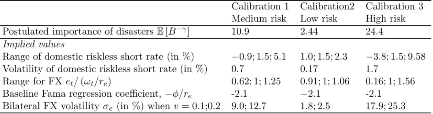
Table 1 presents the main results. In Calibration 1, with v = 0.2, the volatility of the bilateral exchange rate is 11%, and with v = 0.1, 8%. In our low risk calibration (Calibration 2), the corresponding volatilities of the exchange rate are almost trivial: 1.8% and 2.5%. In our high risk calibration (Calibration 3) these volatilities are magnified and become 25.7% and 18.7%, re-spectively. Hence, the model can reasonably generate a high volatility of the exchange rate. The reason is that disasters have a high importance: their importance is magnified byE[B−γ], which is 10.9 (Calibration 1), and 24.4 (Calibration 3). By contrast, in Calibration 2, disasters are milder, risk premia are lower and less volatile, and as a consequence, exchange rates themselves are much smoother.
Table 1: Calibrations of the Model with Medium, Low and High Disaster Risk
Calibration 1 Calibration2 Calibration 3
Medium risk Low risk High risk
Postulated importance of disastersE[B−γ] 10.9 2.44 24.4
Implied values
Range of domestic riskless short rate (in %) −0.9; 1.5; 5.1 1.0; 1.5; 2.3 −3.8; 1.5; 9.58
Volatility of domestic riskless short rate (in %) 0.7 0.17 1.7
Range for FXet/(ωt/re) 0.62; 1; 1.25 0.91; 1; 1.06 0.16; 1; 1.56
Baseline Fama regression coefficient,−φ/re -2.1 −2.1 -2.1
Bilateral FX volatilityσe (in %) when v= 0.1;0.2 9.0; 12.7 1.8; 2.5 17.9; 25.3
Explanation: Each calibration starts with a postulated importance of disasters, E[B−γ]. For instance
if E[B−γ] = 10.9, rare disasters matter 10.9 times as much as they would if agents were risk neutral.
We then fit the rate of time preference δ, to get a typical value of the interest rate close to 1.5%. We
report the minimum, typical (corresponding to Htb = 0) and maximum range for the domestic short
term interest rate; the minimum, typical and maximum value for the exchange rate over “steady state
fundamentals” (ωt/re). Finally, we report for volatility of the bilateral exchange rate for currencies with
two uncorrelated fundamentals. Perfectly correlated currencies have 0 bilateral FX volatility, perfectly
anticorrelated currencies, a volatility equal to the one reported in the table, times √2. The time unit is
the year.
In all three calibrations, the volatility of Ft (defined as Var1/2(Ft+1−Ft)) is 9% per year when
14This is because det et = e Ht r+φ+Het ' e Ht
r+φ, and the bilateral exchange rateeij =ei/ej has twice the variance of any
ν = 0.1, and 12.7% when ν = 0.2: expectations about recovery rate vary pretty rapidly from year to year. AsHbt is quite volatile, the exchange rate is hard to forecast (the same way stocks are hard to forecast). At short horizons, it behaves like a random walk (qualitatively consistent with Meese and Rogoff1983).
In the remaining of this section, we focus on our preferred calibration (Calibration 1) and dig deeper into its implications. We turn to the model’s implications for the correlation between the changes in the exchange rate and the changes in the interest rate. More precisely we are interested in comparingCorr µ ∆(eA t/eBt ) eA t/eBt ,∆ ¡ rA t −rBt ¢
in the data and in the model. In the data, this correlation is close to0. In the simple version of Calibration1we have only one real factor. Hence the correlation is −1 almost by definition. However, a two-factor version of our model similar to that developed in Section 3 performs much better. The reason for this is that although the disaster factor pushes towards a negative correlation, the business cycle factor by contrast, pushes towards a positive correlation. For the purpose of the calibration, it is more intuitive to model business cycle shocks as shocks to productivity trend growth rather than shocks to the level of productivity.15
We choose the average standard deviation of the innovation in bgω,t to be σegω,t = 1.4% and a mean-reversion coefficientφg = 10%. With these numbers, we have
Corr à ∆¡eAt/eBt ¢ eA t/eBt ,∆¡rtA−rtB¢ ! =−0.027.
The volatility of the bilateral exchange is11.1%, the volatility of the domestic interest rate is1.0%. The Fama coefficient is still negative but smaller in absolute value: β0 = −0.04. This of course, is to be anticipated because we have introduced a business-cycle factor with significant variance. To some extent, there is tension in the assumed volatility of the business-cycle factor σˆgω,t, between matching small correlation Corr
µ ∆(eA t/eBt) eA t/eBt ,∆ ¡ rA t −rBt ¢
and generating a large negative Fama regression coefficient.
5
Option prices and exchange rate risk premia
5.1
Theory
Option prices incorporate direct information about the probability and severity of disasters. In particular, consider the implied volatility smile of a pair of currencies: a risky currency and a safe currency. The smile will be much steeper on the risky currency side. A high “smile-skew” should
15More precisely, we assume that productivity growth has deviations from trend,bg ω,t ωt+1 ωt = (1 +bgω,t) exp (gω)× ½ 1 in normal times Ft+1 if disaster
which follows a twisted AR(1) process,Et[bgω,t+1] = 1+1+HH∗t
exp(−φg)egω,t
1+egω,t . Then, Eq. 20 and 21 hold to afirst order,
predict currency appreciation, high interest rate differential and high bond returns.
Consider two countries A andB. The currencyB price at date 0 of a call that gives the option to buy at date1one unit of currencyB forKeB0
eA 0 units of currencyAis 1 eB 0 E0 ∙ M∗ T M∗ 0 ³ eB1 −K eB 0 eA 0 e A 1 ´+¸ , i.e. VCall(K) =E0 " M∗ 1 M∗ 0 µ eB 1 eB 0 −Ke A 1 eA 0 ¶+# . (25)
Likewise, the currency B price at date0of a put that gives the option to sell at date 1one unit of currency B for KeB0 eA 0 units of currencyAis V P ut(K) = E0 ∙ M∗ 1 M∗ 0 ³ KeA1 eA 0 − eB 1 eB 0 ´+¸ .
In order to gain in tractability, we make two simplifying assumptions, as in Gabaix (2007b). First we assume that if a disaster occurs in period t+ 1, εH
t+1 is equal to zero. Second, we assume
that the distribution of et+1 conditional on date t information and no disaster occurring in period t+ 1 is lognormal with drift μi,t and volatilityσi,t where i∈ {A, B} indexes countries: ei,N D1 /ei0 =
exp (μi+εi−σ2i/2)with εi ∼N(0, σ2i).16
Proposition 7 The price of a call with strike K is:
VCall(K) = exp (−R+μB) (1−p0)CBS ¡ Kexp (μA−μB), σA|B ¢ + (26) + exp (−R+μB)p0ED0 £ B1−γ(F1,B −Kexp (μA−μB)F1,A)+ ¤
where CBS(K, σ) is the Black-Scholes call value when the strike is K, the volatility σ, the interest rate 0, the maturity 1, the spot price 1 and
σA|B ≡ ¡ σ2A+σ2B−2ρA,BσAσB ¢1/2 = µ V arN Dln µ eB1 eB 0 /e A 1 eA 0 ¶¶1/2
is the standard deviation of the bilateral log exchange rate if there is no disaster. The price of a put is given by the Put-Call parity equation:
VP ut(K) =VCall(K) + K 1 +rA −
1 1 +rB
(27)
The option price (26) is the sum of two terms. Thefirst one is a familiar Black-Scholes term. The second is a purely disaster term. For strikes close to the spot, the Black-Scholes term dominates. But far out of the money, if the disaster term is not 0, it will typically dominate.
5.2
Risk Reversals
Option prices reveal the risk-neutral distribution — that is, the physical probabilities adjusted for risk— of future exchange rates. Disasters are associated with large movements in exchange rates.
16This can be insured as in Gabaix (2007b). We assume that, if there is no disaster, thenω
t+1/ωt=eg¡1 +εωt+1 ¢ , withEt£εωt+1 ¤ =Et£εωt+1εHt+1 ¤
= 0. This does not change any of the formulas for the exchange rate and the interest rate. The disturbance termεω
t+1 can be designed to insure thate i,N D
Information about disaster risk-premia can logically be extracted from out of the money option prices. Indeed, consider the price of a “risk reversal”:
RR(k)≡ 1 T ∙ VP ut µ 1 +rA 1 +rB k ¶ −VCall µ 1 +rA 1 +rB k−1 ¶¸ (28)
with k > 0, and T is the duration of a “period” in years. This is the price of a put at a fraction
k ≤1of the forward rate, minus the price of a call at a fraction1/k≥1of the forward rate (indeed,
1+rA
1+rB is the forward rate of the currency, as a multiple of the current spot price). If there is a high crash risk for currency B (i.e., currency B will do worse than currency A during disasters), then
RRshould be positive. If there is higher crash risk for currencyA,RR should be negative. If there is no disaster risk, thenRR is very close to0. Risk-reversals are used routinely by traders engaged in currency speculation and in the carry trade in particular as it allows them to bound the gains and losses on their positions.
Calculations show that it is approximately, for short time periods T, and for |k−1| large compared toσAB
√
T (so that the disaster terms mostly influence the value ofRR):
RR'Ψ³HbB−HbA,(1−k)H∗/T ´
(29)
where Ψ(x, y) = (x−y)+−(−x−y)+, a relation that has a shape illustrated in the left panel of Figure 2. The risk reversal position is such that the Black-Scholes component of the put and call have the same price in the limit of short maturities. This allows us to extract the disaster intensities from option prices. When ¯¯¯ bHB−HbA
¯ ¯
¯ is large compared to |1−k|H∗/T,
RR'HbB−HbA. (30)
Hence, the risk reversal is approximately the difference in resilience between the two countries. Conditionally on no disasters, the excess return on a position long on currency B, and short in currency A, is: EN Dt ∙ eB t+T −eBt eB t − eA t+T −eAt eA t ¸ /T +rAt −rtB =HtB−HtA (31) which is close toRR. That is, a currency with a high put price should have a low price, and should subsequently appreciate. This is because it has a high risk premium, that affects both the put value, and a low value of the exchange rate. Equation 31 expresses quantitatively the magnitude of the effect.
5.3
Risk Reversals and Currency Returns
We illustrate the potential power of risk reversals to forecast currency returns. We consider two countries, A and B, with same permanent resilience (HA∗ = HB∗ = H∗), but perhaps different transient resiliences,HbAt,HbBt. We take currencyA’s at its steady state,HbAt = 0. We take a period
0.8 0.9 1.0 1.1 1.2 Strike 0.05 0.10 0.15 0.20 0.25 0.30 Implied Volatility 0.9 1.0 1.1 1.2 Strike 0.15 0.20 0.25 0.30 0.35 Implied Volatility
Figure 1: Implied volatility vs Strike. Units are annualized. CountryB is riskier than country
A. So, the implied volatility of out of the money puts is high. The dotted line is the mirror image of the solid curve, replacing the strikek by its symmetrical value around the forward exchange rate, 1/k. It illustrates that for deep puts, the implied volatility of an out of the money put on currency
B is higher than the implied volatility of an out of the money symmetrical call. The values chosen are: HbA = 0,HbB =−5% in annualized values. Finally, the left panel corresponds to no noise, and the right panel corresponds to a noise ν = 0.5.
length of T equal to 3 months.
At this stage, we need to specify a detail that did not matter before, the volatility of the realiza-tion ofFAin (26): for an option, the uncertainty about the realization of the risk matters. We choose to say that if FA is the expected recovery of country A, its actual realization is FA = FA(1±ν), where the noise ν will be chosen either equal to 0 (no uncertainty) or 0.5 (high uncertainty), no correlations across countries. Given we have no strong prior on the value of that uncertainty, we show the plots for two values. In Figures 1-3, the left panel corresponds to no noise (ν = 0), and the right panel corresponds to a noise ν = 0.5.
Implied volatility and risk reversals. Figure 1 shows the implied volatility of a put as a function of the strike. We take the case where country B is riskier than country A. We take HbB =−5%in annualized values. So, the implied volatility of out of the money puts is high. The dotted line is the mirror image of the solid curve, replacing the strike k by 1/k. It illustrates that for deep puts, implied volatilities of the crash of currencyB are higher than implied volatility of a boom. We see that more noise increase implied volatility, as it should, and also decreases the difference between the put implied volatility (evaluated at k < 1) and the symmetrical call volatility (evaluated at 1/k >1).
Resilience and risk reversals. Figure 2 analyzes the impact of country B’s resilience (HbB) on the value of the risk-reversal, assuming a relative strike k = 0.8. The Figure illustrates that when countryB is riskier, its risk-reversal is more expensive. When there is enough noise, the relation is approximately linear.
Currency returns and risk reversals. Figure 3 plots the expected returns on a position of one unit long of a currencyB bill, and one unit short of currencyA short term bill, vs the risk reversal. We again assume a relative strike k = 0.8. When country B is riskier, its risk-reversal is higher
0.05
0.02
0.05
Resilience
0.02
0.04
Risk Reversal
0.05
0.05
Resilience
0.06
0.04
0.02
0.02
0.04
Risk Reversal
Figure 2: Risk-Reversal vs Resilience. Units are annualized. Thefigure plots the Risk-Reversal (28) vs the resilience HbB, assuming the country A is at the steady state, HbA = 0. The Figure illustrates that when countryB is riskier, its risk-reversal is higher. The left panel corresponds to no noise, and the right panel corresponds to a noise ν = 0.5.
0.05 0.05 Risk Reversal 0.05 0.05 Expected Return 0.05 0.05 Risk Reversal 0.05 0.05 Expected Return
Figure 3: Risk-Reversal vs Expected Returns. Units are annualized. The figure plots the expected returns on a position of 1 unit long of a currency B bill, and 1 unit short of currency A
short term bill, vs the the risk reversal. We assume that country A is at the steady state,HbA = 0. The Figure illustrates that when country B is riskier, its risk-reversal is higher and its expected returns are higher. The left panel corresponds to no noise, and the right panel corresponds to a noise ν = 0.5.
and its expected returns are higher. We see that when the noise is higher, the relation becomes approximately linear as in (30)-(31). Hence, one can hope to use risk-reversals to forecast currency returns. We explore these issues in Farhi, Gabaix, Ranciere and Verdelhan(2008).
5.4
Some Evidence: Contemporaneous Correlations between Currency
Movements and Risk Reversals
Carr and Wu (2007) compute the risk-reversals for two pairs of countries: UK and Japan versus the US. They find a high correlation between changes in the price of risk-reversal options and changes in nominal exchange rates: currencies that become riskier — for which puts become relatively more expensive than calls — experience a simultaneous depreciation. Farhi, Gabaix, Ranciere and Verdelhan (2008) extends their analysis to a sample of 25 countries. Their analysis confirms the finding of Carr and Wu(2007)and shows that it also holds for real exchange rates, providing direct evidence in favor of our model.17
We next turn to two extensions of our model, to nominal rates, and to stocks.
6
Yield curve, forward rates, and exchange rates, real and
nominal
6.1
Exchange rates and long term real rates
To study the forward premium puzzle for long term rates, we first derive the price of long term bonds. The price of a bond yield one unit of the currency at time t+T is: Zt(T) =Et
hM∗ t+Tet+T M∗ tet i .
The yield at maturity T, Yt(T), and the forward ratesft(T)are defined by
Zt(T) = exp (−Yt(T)T) = exp à − T X T0=1 ft(T0) ! .
Proposition 8 (Price of a domestic bond, when there is no inflation on the home goods) The domestic forward rate is, in the continuous time limit, up to second order terms in Hbt and yt,
ft(T) =re−λ− re re+φH exp (−φHT)Hbt+ reφy re+φy exp¡−φyT¢yt (32)
The proof to this Proposition also calculates the expressions for bonds, yields, forward rates, in discrete and continuous time.
The proof is in Appendix B.
17In a contemporaneous paper, Brunnermeier, Nagel and Pedersen (2008) provide an interesting analysis of the
To illustrate the economics, suppose that the country has a very highHbt, i.e. is very safe. Future b
Ht will, on average, mean-revert to 0. Hence, by (11), the exchange rate (which is high now) will depreciate. The short terms rates are low (Eq. 15), which is the forward premium puzzle. Eq. 32 says that long term rates are low (the bond price is high because Hbt.is high). Hence, perhaps paradoxically at first, investors expect the exchange rate to depreciate in the long term, and also, long term rates are low. In the model, this is because investors perceive the country as very “safe”, and require a small risk premium on it.
6.1.1 Fama regression with forward rates
Boudoukh, Richardson and Whitelaw (BRW, 2006) propose to regress the exchange rate movement on the T−period forward rate from T periods ago:
BRW regression: Et ∙eA t+1−eAt eA t −e B t+1−eBt eB t ¸ =αF wd(T)−βF wd(T) (ftA−T (T + 1)−ftB−T (T + 1)) (33) Our model’s prediction is in the next Proposition.
Proposition 9 (Value of the β coefficient in the Fama regression, with two factors, with forward rates). Up to second order terms, in the BRW (33) regression with forward rates, the coefficients are:
βF wd(T) =ν(T)β+ 1−ν(T) (34) and
βF wd,F ull(T) =ν(T)βF ull+ 1−ν(T) (35) where β and βF ull are given in Eqs. 17 and 18, and
ν(T) = ³ re re+φH ´2 Var³Hbt ´ exp (−2φHT) ³ re re+φH ´2 Var³Hbt ´ exp (−2φHT) + ³ r eφy re+φy ´2 Var (yt) exp¡−2φyT ¢ (36)
is the share of variance in the forward rate due toHbt. In particular, whenφH > φy, the long horizon regression have coefficient going to 1: limT→∞βF wd(T) = limT→∞βF wd,F ull(T) = 1.
BRW (2006) find that βf wd(T) increases toward 1 with the horizon. Our theory is consistent with this empirical finding. Indeed, to interpret Proposition 9, consider the case where risk-premia are fast mean-reverting, and productivity is slowly mean reverting, φH > φy. Then, large T, ν(T) tends to 0, which means that, at long horizons, the forward rate is mostly determined by the level of yt, not of the risk premium. Hence, at long horizon the model behaves like a model without risk premia, hence generates a coefficient β close to 1.
6.2
A simple model of exchange rates and nominal yield curves
Until recently, forward real interest rates were not available. Only their nominal counterparts were the support of actively traded securities. Even today, most bonds are nominal bonds.
To model nominal bonds, we build on the real two factor model developed above. Let Qt =
Q0
t Y s=1
(1−is) be the value of money (the inverse of the price level). The nominal interest rate ert satisfies 1+1hr t =Et hM∗ t+1et+1 M∗ tet (1−it) i
, so that, in the continuous time limit, e
rt=rt+it, (37)
the nominal interest rate is the real interest rate, plus inflation. The Fisher neutrality applies: there is no burst of inflation during disasters. With a burst of inflation, even short term bonds would command a risk premium.
Inflation hovers around i∗, according to the LG process:
it+1 =i∗+ 1−i∗
1−it
exp (−φi) (it−i∗) +εit+1 (38)
where εi
t+1 has mean 0, and is uncorrelated with innovations in Mt+1, in particular with disasters.
One could correlate this, but the analysis is a bit more complicated (the analysis is available upon request). The expected value of 1 unit of currency T period later is:
Et ∙ Qt+T Qt ¸ = (1−i∗)T µ 1− 1−exp (−φiT) 1−exp (−φi) it−i∗ 1−i∗ ¶ (39) orEt hQ t+T Qt i = exp (−i∗T)³1− 1−exp(−φiT) φi (it−i∗) ´
in the continuous time limit.
Tofix notations, we denote nominal variables with a tilde. The price of long term nominal bonds yielding one unit of the currency at time t+T is Zet(T) = Et
hM∗ t+Tet+TQt+T M∗ tetQt i . Because we assume that shocks to inflation are uncorrelated with disasters, the value present value of one nominal unit of the currency is e Zt(T) =Et ∙ M∗ t+Tet+TQt+T M∗ tetQt ¸ =Et ∙ M∗ t+Tet+T M∗ tet ¸ Et ∙ Qt+T Qt ¸
Hence, the value of the zero coupon bond is:
Proposition 10 (Price of a nominal domestic bond, with no inflation risk premia) The domestic nominal forward rate is, in the continuous time limit, up to second order terms inHbtand yt,it−i∗ :
ft(T) =re−λ− re re+φH exp (−φHT)Hbt+ reφy re+φy exp¡−φyT¢yt+i∗+ exp (−φiT) (it−i∗) (40)
discrete and continuous time.
The nominal forward rate in (40) depends on real and nominal factors. The real factors are the resilience of the economy (the Hbt) term, the expected growth rate of productivity (−φyyt). The nominal factor is inflationit.
Each of the three terms is multiplied by a term of the type exp (−φHT). For small speeds of mean reversion φ’s, it means that the forward curve is fairly flat.
WithQt the value of money, the nominal exchange rate is: eet =etQt. The expected depreciation of the nominal exchange rate is, up to second order terms, and conditionally on no disasters:
Et ∙ deet e et ¸ /dt=gω− φHHbt re+φH − reφyyt re+φy − it (41)
We can derive the implications of our model for a Fama regression in nominal terms:
Et ∙˜eA t+1−e˜At ˜ eA t − e˜ B t+1−˜eBt ˜ eB t ¸ = ˜αnom−β˜nom(˜rtA−r˜Bt ) (42)
where r˜tA and r˜tB are now, with some a slight abuse of notational, the nominal interest rates in countries A andB. Our model’s prediction is in the next Proposition.
Proposition 11 (Value of theβ coefficient in the Fama regression in nominal terms). Up to second order terms, in the nominal Fama regression (42) regression with forward rates, the coefficients are:
˜
βnom =νnomβ+ 1−νnom and β˜nom,F ull=νnomβF ull+ 1−νnom (43) where β and βF ull are the coefficients in the Fama regression defined in propositions (4) and (??), and νnom = ³ re re+φH ´2 Var³Hbt ´ ³ re re+φH ´2 Var³Hbt ´ +³ reφy re+φy ´2 Var (yt) + Var(it) (44)
is the share of variance in the forward rate due to Hbt.
In this simple model with no inflation risk premia, the higher the variance of inflation , the closer to 1 is βnom. Hence, countries with very variable inflation (typically, those are also countries with high average inflation) satisfy approximately the uncovered interest rate parity conditions. When disaster risks are very variable –and the real exchange rate is very variable — then βnom is more negative.
6.3
A richer model with nominal risk premia
We now develop a richer model with an inflation-specific risk premium. We extend the framework developed in the previous section by incorporating inflation risk along the lines of Gabaix (2007a).
The variable part of inflation now follows the process: bit+1 = 1−i∗ 1−it · ³ exp (−φi)bit+ 1{Disaster att+1} ³ j∗+bjt ´´ +εit+1 (45)
In case of a disaster, inflation jumps by an amount jt = j∗ +bjt. This jump in inflation makes long term bonds particularly risky. j∗ is the baseline jump in inflation, bjt is the mean-reverting deviation from baseline. It follows a twisted auto-regressive process, and, for simplicity, does not jump during crises:
bjt+1 = 1−i∗ 1−it · exp (φπ)bjt+εjt+1 (46) We define πit ≡ pB−γF
1+H bjt, which is the mean-reverting part of the “risk adjusted” expected increase in inflation if there is a disaster. We parametrize the typical jump in inflation j∗ in terms of a numberκ ≤(1−ρi)/2: pB−γF j ∗ 1 +H = (1−i∗) 2 κ(1−ρi−κ).
κ represents a risk premium for the risk that inflation increases during disasters. Also, we define
i�